python logistic回归_softmax回归原理与实现

最新推荐文章于 2024-01-31 16:58:53 发布

weixin_39716264

最新推荐文章于 2024-01-31 16:58:53 发布

阅读量474

点赞数

文章标签： python logistic回归

本文链接：https://blog.csdn.net/weixin_39716264/article/details/111638470

版权

一、什么是 softmax 回归？

softmax 回归(softmax regression)其实是 logistic 回归的一般形式，logistic 回归用于二分类，而 softmax 回归用于多分类，关于 logistic 回归可以看我的这篇博客

小胡子：机器学习-logistic回归原理与实现zhuanlan.zhihu.com

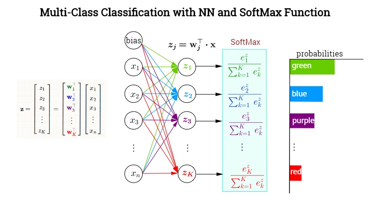
对于输入数据

有

个类别，即

，那么 softmax 回归主要估算输入数据

归属于每一类的概率，即

其中，

是模型的参数，乘以

是为了让概率位于[0,1]并且概率之和为 1，softmax 回归将输入数据

归属于类别

的概率为

上面的式子可以用下图形象化的解析(来自台大李宏毅《一天搞懂深度学习》)。

二、原理

2.1 梯度下降法参数求解

softmax 回归的参数矩阵

可以记为

定义 softmax 回归的代价函数

其中，1{·}是示性函数，即1{值为真的表达式}=1，1{值为假的表达式}=0。跟 logistic 函数一样，利用梯度下降法最小化代价函数，下面求解

的梯度。

关于

的梯度求解为

感谢 CSDN 博主[2]提供了另外一种求解方法，具体如下

2.2 模型参数特点

softmax 回归有一个不寻常的特点：它有一个“冗余“的参数集。为了便于阐述这一特点，假设我们从参数向量

中减去向量

，那么对于概率函数，我们有

换句话说，从参数向量中的每个元素

中减去

一点也不会影响到假设的类别预测！这表明了 softmax 回归的参数中是有多余的。正式地说， softmax 模型是过参数化的（ overparameterized 或参数冗余的），这意味着对任何一个拟合数据的假设而言，多种参数取值有可能得到同样的假设

，即从输入

经过不同的模型参数的假设计算从而得到同样的分类预测结果。

进一步说，若代价函数

被某组模型参数

最小化，那么对任意的

，代价函数也可以被

最小化。因此，

的最小值时的参数并不唯一。（有趣的是，

仍是凸的，并且在梯度下降中不会遇到局部最优的问题，但是 Hessian 矩阵是奇异或不可逆的，这将会导致在牛顿法的直接实现上遇到数值问题。）

注意到，通过设定

，总是可以用

代替

，而不会对假设函数有任何影响。因此，可以去掉参数向量

中的最后一个（或该向量中任意其它任意一个）元素

，而不影响假设函数的表达能力。实际上，因参数冗余的特性，与其优化全部的

个参数

（其中

），也可令

，只优化剩余的

个参数，算法依然能够正常工作。

2.3 正则化

当训练数据不够多的时候，容易出现过拟合现象，拟合系数往往非常大 [过拟合原因]，为此在损失函数后面加上一个正则项，即

那么新的损失函数的梯度为

⚠️注意：上式中的

中的

不应该被惩罚，因为他是一个常数项，所以在实际使用的时候仅仅需要对

进行惩罚即可，这个会在后面的 python 代码中提到。

2.4 softmax 与 logistic 回归的关系

文章开头说过，softmax 回归是 logistic 回归的一般形式，logistic 回归是 softmax 回归在

时的特殊形式，下面通过公式推导来看下当

时 softmax 回归是如何退化成 logistic 回归。

当

时，softmax 回归的假设函数为

前面说过 softmax 回归的参数具有冗余性，从参数向量

中减去向量

完全不影响结果。现在我们令

，并且两个参数向量都减去

，则有

这样就化成了 logistic 回归。

三、实现

3.1 python 手动实现

这里的数据使用的是 sklearn 的算法包生成的随机数据，其中，训练数据为 3750×2 的数据，测试数据为 1250×2 的数据，生成代码如下

def gen_dataset():
    from sklearn.datasets import load_iris
    from sklearn.model_selection import train_test_split
    from sklearn.datasets import make_blobs
    import matplotlib.pyplot as plt
    np.random.seed(13)
    X, y = make_blobs(centers=4, n_samples = 5000)
    # 绘制数据分布
    plt.figure(figsize=(6,4))
    plt.scatter(X[:,0], X[:,1],c=y)
    plt.title("Dataset")
    plt.xlabel("First feature")
    plt.ylabel("Second feature")
    plt.show()

    # 重塑目标以获得具有 (n_samples, 1)形状的列向量
    y = y.reshape((-1,1))
    # 分割数据集
    X_train, X_test, y_train, y_test = train_test_split(X, y)
    train_dataset = np.append(X_train,y_train, axis = 1)
    test_dataset = np.append(X_test,y_test, axis = 1)
    np.savetxt("train_dataset.txt", train_dataset, fmt="%.4f %.4f %d")
    np.savetxt("test_dataset.txt", test_dataset, fmt="%.4f %.4f %d")

数据分布情况如下图所示

softmax 算法的核心部分就是求解梯度矩阵，我们设输入数据为

，这是一个

的矩阵，输出类别为

，其中

是一个

的one-hot 矩阵，

表示类别个数，那么

其实是一个

的矩阵，输入数据对应的概率为

，同样的这也是一个

的矩阵。那么根据公式(9)，可以知道

的梯度为

由此可以推导出

的参数矩阵为

注意到这里也考虑了

的第 0 项，所以在写代码的时候需要把

的第 0 列的惩罚项减去。

softmax 回归的代码如下

def load_dataset(file_path):
    dataMat = []
    labelMat = []
    fr = open(file_path)
    for line in fr.readlines():
        lineArr = line.strip().split()
        dataMat.append([1.0, float(lineArr[0]), float(lineArr[1])])
        labelMat.append(int(lineArr[2]))
    return dataMat, labelMat


def train(data_arr, label_arr, n_class, iters = 1000, alpha = 0.1, lam = 0.01):
    '''
    @description: softmax 训练函数
    @param {type} 
    @return: theta 参数
    '''    
    n_samples, n_features = data_arr.shape
    n_classes = n_class
    # 随机初始化权重矩阵
    weights = np.random.rand(n_class, n_features)
    # 定义损失结果
    all_loss = list()
    # 计算 one-hot 矩阵
    y_one_hot = one_hot(label_arr, n_samples, n_classes)
    for i in range(iters):
        # 计算 m * k 的分数矩阵
        scores = np.dot(data_arr, weights.T)
        # 计算 softmax 的值
        probs = softmax(scores)
        # 计算损失函数值
        loss = - (1.0 / n_samples) * np.sum(y_one_hot * np.log(probs))
        all_loss.append(loss)
        # 求解梯度
        dw = -(1.0 / n_samples) * np.dot((y_one_hot - probs).T, data_arr) + lam * weights
        dw[:,0] = dw[:,0] - lam * weights[:,0]
        # 更新权重矩阵
        weights  = weights - alpha * dw
    return weights, all_loss
        

def softmax(scores):
    # 计算总和
    sum_exp = np.sum(np.exp(scores), axis = 1,keepdims = True)
    softmax = np.exp(scores) / sum_exp
    return softmax


def one_hot(label_arr, n_samples, n_classes):
    one_hot = np.zeros((n_samples, n_classes))
    one_hot[np.arange(n_samples), label_arr.T] = 1
    return one_hot


def predict(test_dataset, label_arr, weights):
    scores = np.dot(test_dataset, weights.T)
    probs = softmax(scores)
    return np.argmax(probs, axis=1).reshape((-1,1))


if __name__ == "__main__":
    #gen_dataset()
    data_arr, label_arr = load_dataset('train_dataset.txt')
    data_arr = np.array(data_arr)
    label_arr = np.array(label_arr).reshape((-1,1))
    weights, all_loss = train(data_arr, label_arr, n_class = 4)

    # 计算预测的准确率
    test_data_arr, test_label_arr = load_dataset('test_dataset.txt')
    test_data_arr = np.array(test_data_arr)
    test_label_arr = np.array(test_label_arr).reshape((-1,1))
    n_test_samples = test_data_arr.shape[0]
    y_predict = predict(test_data_arr, test_label_arr, weights)
    accuray = np.sum(y_predict == test_label_arr) / n_test_samples
    print(accuray)

    # 绘制损失函数
    fig = plt.figure(figsize=(8,5))
    plt.plot(np.arange(1000), all_loss)
    plt.title("Development of loss during training")
    plt.xlabel("Number of iterations")
    plt.ylabel("Loss")
    plt.show()

函数输出的测试数据准确率为

0.9952

程序中记录了每个循环的损失函数，其变化曲线如下图所示。

3.2 sklearn 算法包实现

sklearn的实现比较简单，与 logistic 回归的代码类似。

def softmax_lib():
    data_arr, label_arr = load_dataset('train_dataset.txt')
    from sklearn import linear_model
    model_softmax_regression = linear_model.LogisticRegression(solver='lbfgs',multi_class="multinomial",max_iter=10)
    model_softmax_regression.fit(data_arr, label_arr)
    test_data_arr, test_label_arr = load_dataset('test_dataset.txt')
    y_predict = model_softmax_regression.predict(test_data_arr)
    accurcy = np.sum(y_predict == test_label_arr) / len(test_data_arr)
    print(accurcy)

输出结果为

0.9848

本文的完整代码和数据去 [我的 github]查看

四、参考

[1]

帅帅家的人工智障：常见机器学习算法实现 7 之Softmax 回归zhuanlan.zhihu.com

[2]

https://blog.csdn.net/u012328159/article/details/72155874blog.csdn.net

[3]

素轻：Hierarchical Softmax（层次Softmax）zhuanlan.zhihu.com

[4]

https://zh.wikipedia.org/wiki/Softmax%E5%87%BD%E6%95%B0zh.wikipedia.org

[5]

Unsupervised Feature Learning and Deep Learning Tutorialdeeplearning.stanford.edu

weixin_39716264

关注

0
点赞
踩
0

收藏

觉得还不错? 一键收藏
0
评论
python logistic回归_softmax回归原理与实现

一、什么是 softmax 回归？softmax 回归(softmax regression)其实是 logistic 回归的一般形式，logistic 回归用于二分类，而 softmax 回归用于多分类，关于 logistic 回归可以看我的这篇博客小胡子：机器学习-logistic回归原理与实现zhuanlan.zhihu.com对于输入数据有个类别，即，那么 softmax 回归主...
复制链接

扫一扫