arma模型_ARMA模型的两套图

ARMA类模型常用的两套图，一是验证平稳性的特征根与单位圆的关系，二是ACF和PACF。对于前者，MMA可以帮我们计算特征根；对于后者，ACF和PACF有现成的函数计算理论值，而非模拟序列的样本自相关和样本偏自相关函数。

一、特征根和单位圆

举例：对于AR(3)模型 u_t= 0.6*u_{t-1} + 0.3*u_{t-2}+0.1*u_{t-3}+e_t

sol = Solve[1 - 0.6 x - 0.3 x^2 - 0.1 x^3 == 0, x]x /. sol // Abs

可得到三个根，其中一个是单位根：

{{x -> -2. - 2.44949 I}, {x -> -2. + 2.44949 I}, {x -> 1.}}

只有前两个满足模条件：

{3.16228, 3.16228, 1.}

作图可以看到这个u序列是非平稳的：

p1 = ComplexListPlot[x /. sol2, PlotRange -> {{-3, 3}, {-3, 3}},    PlotStyle -> Directive[PointSize[Large], Red]];p2 = ParametricPlot[{r Cos[\[Theta]], r Sin[\[Theta]]}, {\[Theta], 0,     2 Pi}, {r, 0, 1}];Show[p1, p2]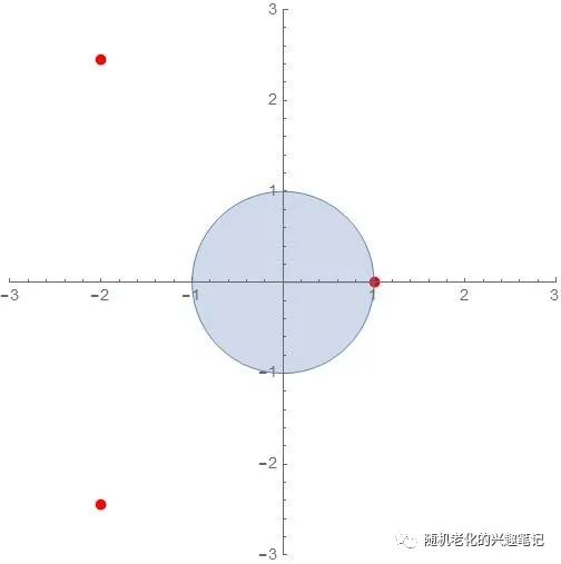

二、ACF和PACF

举例：(将前面的模型的一个参数作个修改演示)

对于AR(3)模型 u_t= -0.6*u_{t-1} + 0.3*u_{t-2}+0.1*u_{t-3}+e_t

ListPlot[CorrelationFunction[ARProcess[{-.6, .3, .1}, 4], {20}],  Filling -> Axis, PlotRange -> All, Mesh -> All, Joined -> True,  Frame -> True, MeshStyle -> Directive[PointSize[Medium], Red],  PlotLabel ->   "\!\(\*SubscriptBox[\(u\), \(t\)]\)=-0.6\!\(\*SubscriptBox[\(u\), \\(t - 1\)]\)+0.3\!\(\*SubscriptBox[\(u\), \(t - \2\)]\)+0.1\!\(\*SubscriptBox[\(u\), \(t - \3\)]\)+\!\(\*SubscriptBox[\(\[Epsilon]\), \\(t\)]\),\!\(\*SuperscriptBox[\(\[Sigma]\), \(2\)]\)=4的ACF图"]ListPlot[PartialCorrelationFunction[  ARProcess[{-.6, .3, .1}, 4], {20}], Filling -> Axis,  PlotRange -> All, Mesh -> All, Joined -> True, Frame -> True,  MeshStyle -> Directive[PointSize[Medium], Red],  PlotLabel ->   "\!\(\*SubscriptBox[\(u\), \(t\)]\)=-0.6\!\(\*SubscriptBox[\(u\), \\(t - 1\)]\)+0.3\!\(\*SubscriptBox[\(u\), \(t - \2\)]\)+0.1\!\(\*SubscriptBox[\(u\), \(t - \3\)]\)+\!\(\*SubscriptBox[\(\[Epsilon]\), \\(t\)]\),\!\(\*SuperscriptBox[\(\[Sigma]\), \(2\)]\)=4的PACF图"]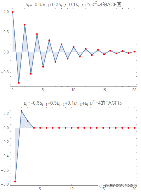

可以看到自回归模型在ACF上的拖尾性和在PACF上的截尾性。

当然也可以做MA过程和ARMA过程，只是把函数名改一下即可，这里就不浪费空间了。