circle loss代码实现_梯度下降迭代更新多元线性回归参数的Numpy实现

引言

梯度下降作为目前非线性预测模型(随机森林、支持向量机、神经网络、深度学习等)的主流参数更新方法，鲜有在线性回归模型中进行利用。主要原因笔者认为有以下两点:一方面，归功于非线性模型超高的模型拟合优度以及分类精度。另一方面，解析法求解线性模型参数的方式已广泛地被学者们认可。但是，这并不意味着线性模型的发展停滞不前，线性模型的计算复杂度低，效率高，在预测领域仍然具有较高的探索价值。因此，为了更好地优化线性模型，本文章将带大家实现梯度下降方法的多元线性回归参数的更新迭代。

代码实现流程

• 加载数据和数据归一化
• 超参数设置和模型训练
• 打印loss
• 模型预测

基本原理

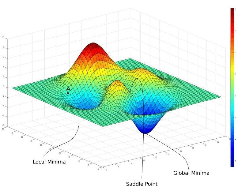
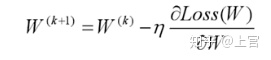
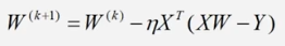
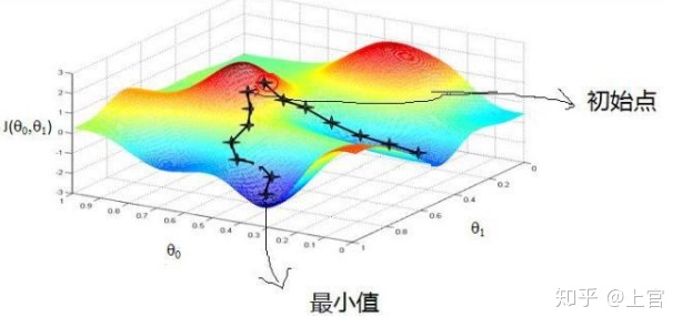
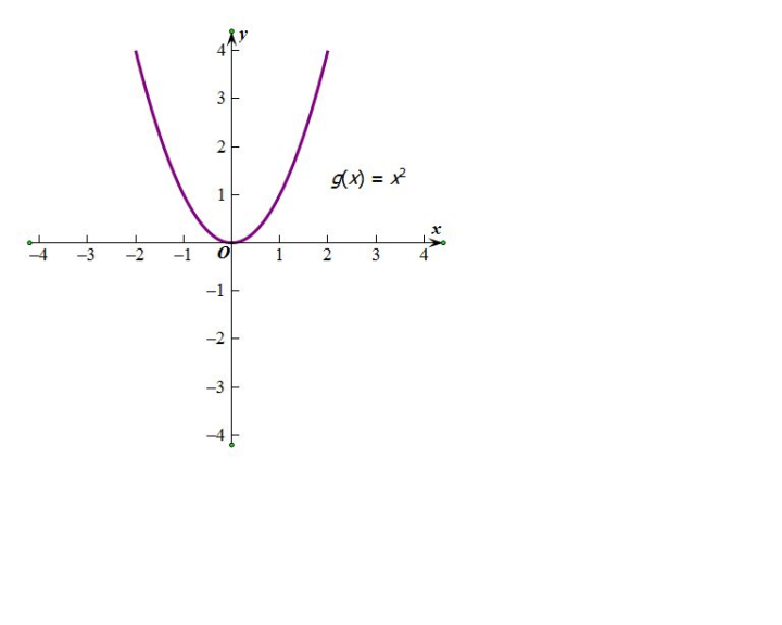
要想实现梯度下降，首先要满足一个前提条件。模型的损失函数必须是一个凸函数，这个凸函数可以是二维也可以是三维。顾名思义，我们所要求的凸函数就是满足我们在函数中找到极小值的需要，这个极小值是全局意义上的极小值。此时，通过设置较小的学习率和充足的迭代数就可以找到这个极小值。对loss函数的参数求解偏导数后，带入权值更新公式中，可以得到最终的更新迭代公式。

权值更新公式

带入偏导数后的公式

梯度下降示意图

数据介绍

本文章所使用的数据为地面高光谱反射率与土壤实测有机质，共一百个样本，测试30个，训练70个。选用五个波段作为自变量，SOM作为因变量。本数据由笔者所在实验室大神---孟XT---辛勤整理并提供，此处作特别鸣谢O(∩_∩)O。

Python代码实现(模型训练)

import numpy as np
import matplotlib.pyplot as plt
import pandas as pd

plt.rcParams["font.sans-serif"] = ["SimHei"]

#数据加载与格式转换
FilePath = r"E:yynctryedata孟PP_训练.xlsx"
origin_data = pd.read_excel(FilePath, sheet_name = 0)
data = np.array(origin_data)

#赋值自变量
B1 = data[:,1]
B2 = data[:,2]
B3 = data[:,3]
B4 = data[:,4]
B5 = data[:,5]

#赋值因变量
SOM = data[:,0]

num = len(B1)

#数据处理
x0 = np.ones(num)

B1 = (B1 - B1.min()) / (B1.max() - B1.min())
B2 = (B2 - B2.min()) / (B2.max() - B2.min())
B3 = (B3 - B3.min()) / (B3.max() - B3.min())
B4 = (B4 - B4.min()) / (B4.max() - B4.min())
B5 = (B5 - B5.min()) / (B5.max() - B5.min())

X_train = np.stack((x0, B1, B2, B3, B4, B5), axis = 1)
Y_train = SOM.reshape(-1, 1)
print(X_train.shape)
print(Y_train.shape)

#超参数设置
learn_rate = 0.001
iter = 1000
display_step = 50

#赋值参数初值
np.random.seed(612)
W = np.random.randn(6, 1)

#模型训练
mse = []
W_set = []
for i in range(0, iter+1):
    dw = np.matmul(np.transpose(X_train), np.matmul(X_train, W)-Y_train) #参数求偏导
    W = W - learn_rate*dw #参数更新
    predict = np.matmul(X_train,W) #预测
    Loss = np.mean(np.square(Y_train - predict))/2 #求损失值
    mse.append(Loss)
    W_set.append(W)

    if i % display_step == 0:
        print("i: %i, Loss:%f" % (i,mse[i]))
    if i % display_step == 0:
        print(W_set[i])

#运行结果可视化
plt.figure(figsize = (12,4))

plt.subplot(1,2,1)
plt.plot(mse)
plt.xlabel("Iteration", fontsize = 14)
plt.ylabel("Loss", fontsize = 14)

plt.subplot(1,2,2)
predict = predict.reshape(-1)
plt.plot(SOM, color = "red", marker = "o", label = "SOM实测值")
plt.plot(predict, color = "blue", marker = ".", label = "SOM预测值")
plt.xlabel("Sample", fontsize = 14)
plt.ylabel("SOM", fontsize = 14)

plt.legend()
plt.show()

Python代码实现(模型预测)

#模型预测
FilePath1 = r"E:yynctryedata孟PP_测试.xlsx"
origin_data1 = pd.read_excel(FilePath1, sheet_name = 0)
data1 = np.array(origin_data1)

#赋值自变量
B1_1 = data1[:,1]
B2_1 = data1[:,2]
B3_1 = data1[:,3]
B4_1 = data1[:,4]
B5_1 = data1[:,5]

#归一化操作
num1 = len(B1_1)
x1 = np.ones(num1)

B1_1 = (B1_1 - B1_1.min()) / (B1_1.max() - B1_1.min())
B2_1 = (B2_1 - B2_1.min()) / (B2_1.max() - B2_1.min())
B3_1 = (B3_1 - B3_1.min()) / (B3_1.max() - B3_1.min())
B4_1 = (B4_1 - B4_1.min()) / (B4_1.max() - B4_1.min())
B5_1 = (B5_1 - B5_1.min()) / (B5_1.max() - B5_1.min())

X_test = np.stack((x1, B1_1, B2_1, B3_1, B4_1, B5_1), axis = 1)
predict_test = np.matmul(X_test,W)

#预测数据输出
data = pd.DataFrame(predict_test)
writer = pd.ExcelWriter(r"E:yynctryedata孟PP_模型预测.xlsx")# 写入Excel文件
data.to_excel(writer, 'page_1', float_format='%.5f')# ‘page_1’是写入excel的sheet名
writer.save()
writer.close()

代码关键点说明：

因为本数据在迭代1000次时Loss达到最小，因此直接用训练代码中的的W进行预测。

运行结果

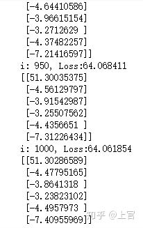
代码会自动生成每50次迭代所对应的Loss值与模型参数:

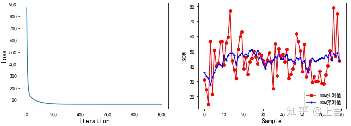
现在我们把模型训练过程中的Loss和预测与实测之间的数据用图表展示出来：

参考文献

梯度下降算法详解​baijiahao.baidu.com

深度技术宅：详解梯度下降法（干货篇）​zhuanlan.zhihu.com

什么是梯度下降法？​www.zhihu.com