bagging和时间序列预测_Simple RNN时间序列预测

本文将介绍利用朴素的RNN模型进行时间序列预测

比方说现在我们有如下图所示的一段正弦曲线，输入红色部分，通过训练输出下一段的值

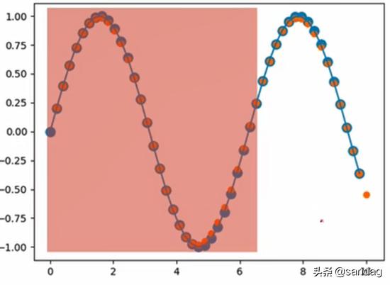
首先分析一下，假设我们一次输入50个点，batch设为1，每个点就一个值，所以input的shape就是 [50, 1, 1] ，这里我们换一种表示形式，把batch放在前面，那么shape就是 [1, 50, 1] ，可以这么理解这个shape，1条曲线，一共有50个点，每个点都是1个实数

import numpy.random import randintimport numpy as npimport torchfrom torch import nn, optimfrom matplotlib import pyplot as pltstart = randint(3) # [0, 3)time_steps = np.linspace(start, start + 10, num_time_steps) # 返回num_time_steps个点data = np.sin(time_steps) # [50]data = data.reshape(num_time_steps, -1) # [50, 1]x = torch.tensor(data[:-1]).float().view(1, num_time_steps - 1, 1) # 0~48y = torch.tensor(data[1:]).float().view(1, num_time_steps - 1, 1) # 1~49

start 表示的含义从几何上来说就是图上红色左边框的对应的横坐标的值，因为我们要确定一个起点，从这个起点开始向后取50个点，如果每次这个起点都是相同的，就会被这个网络记住

x 是50个数据点中的前49个，我们利用这49个点，每个点都向后预测一个单位的数据，得到^yy^，然后将^yy^与yy进行对比

接下来是构建网络架构

class Net(nn.Module):    def __init__(self):        super(Net, self).__init__()        self.rnn = nn.RNN(            input_size=input_size,            hidden_size=hidden_size,            num_layers=1,            batch_first=True,        )        self.linear = nn.Linear(hidden_size, output_size)    def forward(self, x, h0):        out, h0 = self.rnn(x, h0)        # [b, seq, h] => [seq, h]        out = out.view(-1, hidden_size)        out = self.linear(out) # [seq, h] => [seq, 1]        out = out.unsqueeze(dim=0) # => [1, seq, 1]        return out, h0

首先里面是一个simple RNN，其中有个参数 batch_first ，因为我们数据传入的格式是batch在前，所以要把这个参数设为True。RNN之后接了个Linear，将memory的size输出为 output_size=1 方便进行比较，因为我们就只需要一个值

然后我们定义网络Train的代码

model = Net()criterion = nn.MSELoss()optimizer = optim.Adam(model.parameters(), lr)h0 = torch.zeros(1, 1, hidden_size) # [b, 1, hidden_size]for iter in range(6000):    start = np.random.randint(3, size=1)[0]    time_steps = np.linspace(start, start + 10, num_time_steps)    data = np.sin(time_steps)    data = data.reshape(num_time_steps, 1)    x = torch.tensor(data[:-1]).float().view(1, num_time_steps - 1, 1)    y = torch.tensor(data[1:]).float().view(1, num_time_steps - 1, 1)    output, h0 = model(x, h0)    h0 = h0.detach()    loss = criterion(output, y)    model.zero_grad()    loss.backward()    optimizer.step()    if iter % 100 == 0:        print("Iteration: {} loss {}".format(iter, loss.item()))

最后是Predict的部分

predictions = []input = x[:, 0, :]for _ in range(x.shape[1]):    input = input.view(1, 1, 1)    (pred, h0) = model(input, h0)    input = pred    predictions.append(pred.detach().numpy().ravel()[0])

假设 x 的shape是 [b, seq, 1] ，经过 x[:, 0, :] 之后就变成了 [b, 1] ，但其实前面说过了，batch值是1，所以input的shape就是 [1, 1] ，然后再展开成 [1, 1, 1] 是为了能匹配网络的输入维度

倒数第二行和第三行的代码做的事情是，首先带入第一个值，得到一个输出 pred ，然后把 pred 作为下一次的输入，又得到一个 pred ，如此循环往复，就把上一次的输出，作为下一次的输入

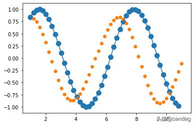
最后的输出图像如下所示

完整代码如下：

from numpy.random import randintimport numpy as npimport torchimport torch.nn as nnimport torch.optim as optimfrom matplotlib import pyplot as pltnum_time_steps = 50input_size = 1hidden_size = 16output_size = 1lr=0.01class Net(nn.Module):    def __init__(self):        super(Net, self).__init__()        self.rnn = nn.RNN(            input_size=input_size,            hidden_size=hidden_size,            num_layers=1,            batch_first=True,        )        self.linear = nn.Linear(hidden_size, output_size)    def forward(self, x, h0):        out, h0 = self.rnn(x, h0)        # [b, seq, h]        out = out.view(-1, hidden_size)        out = self.linear(out)        out = out.unsqueeze(dim=0)        return out, h0model = Net()criterion = nn.MSELoss()optimizer = optim.Adam(model.parameters(), lr)h0 = torch.zeros(1, 1, hidden_size)for iter in range(6000):    start = randint(3)    time_steps = np.linspace(start, start + 10, num_time_steps)    data = np.sin(time_steps)    data = data.reshape(num_time_steps, 1)    x = torch.tensor(data[:-1]).float().view(1, num_time_steps - 1, 1)    y = torch.tensor(data[1:]).float().view(1, num_time_steps - 1, 1)    output, h0 = model(x, h0)    h0 = h0.detach()    loss = criterion(output, y)    model.zero_grad()    loss.backward()    optimizer.step()    if iter % 100 == 0:        print("Iteration: {} loss {}".format(iter, loss.item()))start = randint(3)time_steps = np.linspace(start, start + 10, num_time_steps)data = np.sin(time_steps)data = data.reshape(num_time_steps, 1)x = torch.tensor(data[:-1]).float().view(1, num_time_steps - 1, 1)y = torch.tensor(data[1:]).float().view(1, num_time_steps - 1, 1)predictions = []input = x[:, 0, :]for _ in range(x.shape[1]):    input = input.view(1, 1, 1)    (pred, h0) = model(input, h0)    input = pred    predictions.append(pred.detach().numpy().ravel()[0])x = x.data.numpy().ravel() # flatten操作y = y.data.numpy()plt.scatter(time_steps[:-1], x.ravel(), s=90)plt.plot(time_steps[:-1], x.ravel())plt.scatter(time_steps[1:], predictions)plt.show()