


pandas常用统计方法
假设现在我们有一组从2006年到2016年1000部最流行的电影数据,我们想知道这些电影数据中评分的平均分,导演的人数等信息,我们应该怎么获取?
数据来源:https://www.kaggle.com/damianpanek/sunday-eda/data
import pandas as pd
from matplotlib import pyplot as plt
import numpy as np

file_path = "./IMDB-Movie-Data.csv"
df = pd.read_csv(file_path)

# 获取平均分
print(df["Rating"].mean())

# 导演的人数
# print(len(set(df["Director"].tolist())))
print(len(df["Director"].unique()))

# 获取演员人数
temp_actors_list = df["Actors"].str.split(", ").tolist()
actors_list = [i for j in temp_actors_list for i in j]
actors_num = len(set(actors_list))
print(actors_num)
运行结果
6.723199999999999
644
2015
常用统计方法
# 评分的平均分
rating_mean = df["Rating"].mean()

# 导演的人数
temp_list = df["Actors"].str.split(",").tolist()
nums = set([i for j in temp_list for i in j])

# 电影的时长的最大值最小值
max_runtime = df["Runtime (Minutes)"].max()
max_runtime_index = df["Runtime (Minutes)"].argmax()
min_runtime = df["Runtime (Minutes)"].min()
min_runtime_index = df["Runtime (Minutes)"].argmin()
runtime_median = df["Runtime (Minutes)"].median()
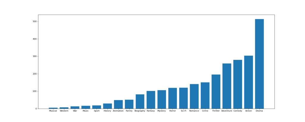
对于这一组电影数据,如果我们希望统计电影分类(genre)的情况,应该如何处理数据?
思路:重新构造一个全为0的数组,列名为分类,如果某一条数据中分类出现过,就让0变为1
import pandas as pd
from matplotlib import pyplot as plt
import numpy as np

file_path = "./IMDB-Movie-Data.csv"
df = pd.read_csv(file_path)

# 统计分类的列表
temp_list = df["Genre"].str.split(",").tolist()  # [[], [], []]

genre_list = list(set([i for j in temp_list for i in j]))

# 构造全为0的数组
zeros_df = pd.DataFrame(np.zeros((df.shape[0], len(genre_list))), columns=genre_list)

# 给每个电影出现的分类位置赋值1
for i in range(df.shape[0]):
    # zeros_df.loc[0, ["Sci-fi", "Music"]] = 1
    zeros_df.loc[i, temp_list[i]] = 1

# print(zeros_df.head(3))

# 统计每个分类的电影的数量和
genre_count = zeros_df.sum(axis=0)
print(genre_count)

# 排序
genre_count = genre_count.sort_values()
_x = genre_count.index
_y = genre_count.values
# 画图
plt.figure(figsize=(20, 8), dpi=80)
plt.bar(range(len(_x)), _y)
plt.xticks(range(len(_x)), _x)
plt.savefig("./t1.png")
数据合并之join
join:默认情况下他是把行索引相同的数据合并到一起
In [66]: t2 = pd.DataFrame(np.zeros((2,5)), index=list(string.ascii_uppercase[:2]), columns=list(string.ascii_uppercase[-5:]))

In [67]: t2
Out[67]:
     V    W    X    Y    Z
A  0.0  0.0  0.0  0.0  0.0
B  0.0  0.0  0.0  0.0  0.0

In [68]: t1 = pd.DataFrame(np.ones((3, 4)), index=list(string.ascii_uppercase[:3]), columns=list(range(0, 4)))

In [69]: t1
Out[69]:
     0    1    2    3
A  1.0  1.0  1.0  1.0
B  1.0  1.0  1.0  1.0
C  1.0  1.0  1.0  1.0

In [70]: t1.join(t2)
Out[70]:
     0    1    2    3    V    W    X    Y    Z
A  1.0  1.0  1.0  1.0  0.0  0.0  0.0  0.0  0.0
B  1.0  1.0  1.0  1.0  0.0  0.0  0.0  0.0  0.0
C  1.0  1.0  1.0  1.0  NaN  NaN  NaN  NaN  NaN
数据合并之merge
merge:按照指定的列把数据按照一定的方式合并到一起
In [113]: t1
Out[113]:
     M    N  O    P
A  1.0  1.0  a  1.0
B  1.0  1.0  b  1.0
C  1.0  1.0  c  1.0

In [114]: t2
Out[114]:
     V    W  X    Y    Z
A  0.0  0.0  c  0.0  0.0
B  0.0  0.0  d  0.0  0.0

In [115]: t = t1.merge(t2, left_on="O", right_on="X")

In [116]: t1
Out[116]:
     M    N  O    P
A  1.0  1.0  a  1.0
B  1.0  1.0  b  1.0
C  1.0  1.0  c  1.0

In [117]: t2
Out[117]:
     V    W  X    Y    Z
A  0.0  0.0  c  0.0  0.0
B  0.0  0.0  d  0.0  0.0

In [118]: t1.merge(t2, left_on="O", right_on="X")
Out[118]:
     M    N  O    P    V    W  X    Y    Z
0  1.0  1.0  c  1.0  0.0  0.0  c  0.0  0.0

In [119]: t1.merge(t2, left_on="O", right_on="X", how="inner")
Out[119]:
     M    N  O    P    V    W  X    Y    Z
0  1.0  1.0  c  1.0  0.0  0.0  c  0.0  0.0

In [120]: t1.merge(t2, left_on="O", right_on="X", how="outer")
Out[120]:
     M    N    O    P    V    W    X    Y    Z
0  1.0  1.0    a  1.0  NaN  NaN  NaN  NaN  NaN
1  1.0  1.0    b  1.0  NaN  NaN  NaN  NaN  NaN
2  1.0  1.0    c  1.0  0.0  0.0    c  0.0  0.0
3  NaN  NaN  NaN  NaN  0.0  0.0    d  0.0  0.0

In [121]: t1.merge(t2, left_on="O", right_on="X", how="left")
Out[121]:
     M    N  O    P    V    W    X    Y    Z
0  1.0  1.0  a  1.0  NaN  NaN  NaN  NaN  NaN
1  1.0  1.0  b  1.0  NaN  NaN  NaN  NaN  NaN
2  1.0  1.0  c  1.0  0.0  0.0    c  0.0  0.0

In [122]: t1.merge(t2, left_on="O", right_on="X", how="right")
Out[122]:
     M    N    O    P    V    W  X    Y    Z
0  1.0  1.0    c  1.0  0.0  0.0  c  0.0  0.0
1  NaN  NaN  NaN  NaN  0.0  0.0  d  0.0  0.0
pandas的分组和聚合
现在我们有一组关于全球星巴克店铺的统计数据,如果我想知道美国的星巴克数量和中国的哪个多,或者我想知道中国每个省份星巴克的数量的情况,那么应该怎么办?
数据来源:https://www.kaggle.com/starbucks/store-locations/data
思路:遍历一遍,每次加1 ???
在pandas中类似的分组的操作我们有很简单的方式来完成df.groupby(by=”columns_name”)
那么问题来了,调用groupby方法之后返回的是什么内容?
grouped = df.groupby(by=”columns_name”)grouped是一个DataFrameGroupBy对象,是可迭代的grouped中的每一个元素是一个元组元组里面是(索引(分组的值),分组之后的DataFrame)
那么,回到之前的问题:要统计美国和中国的星巴克的数量,我们应该怎么做?分组之后的每个DataFrame的长度?
长度是一个思路,但是我们有更多的方法(聚合方法)来解决这个问题
| 函数名 | 说明 |
|---|---|
| count | 分组中非NA值的数量 |
| sum | 非NA值的和 |
| mean | 非NA值的平均值 |
| median | 非NA值的算术中位数 |
| std、var | 无偏(分母为n-1)标准差和方差 |
| min、max | 非NA值的最小值和最大值 |
如果我们需要对国家和省份进行分组统计,应该怎么操作呢?
grouped = df.groupby(by=[df[“Country”],df[“State/Province”]])
很多时候我们只希望对获取分组之后的某一部分数据,或者说我们只希望对某几列数据进行分组,这个时候我们应该怎么办呢?
获取分组之后的某一部分数据:
df.groupby(by=[“Country”,”State/Province”])[“Country”].count()
对某几列数据进行分组:
df[“Country”].groupby(by=[df[“Country”],df[“State/Province”]]).count()
import pandas as pd
import numpy as np

file_path = "./starbucks_store_worldwide.csv"

df = pd.read_csv(file_path)
# print(df.head(1))
# print(df.info())
grouped = df.groupby(by="Country")

# DataFrameGroupBy
# 可以进行遍历
# for i, j in grouped:
#     print(i)
#     print("-" * 100)
#     print(j, type(j))
#     print("*" * 100)
# df[df["Country"]="US"]
# 调用聚合方法
# country_count = grouped["Brand"].count()
# print(country_count["US"])
# print(country_count["CN"])

# 统计中国每个省店铺的数量
# china_data = df[df["Country"] == "CN"]
#
# grouped = china_data.groupby(by="State/Province").count()["Brand"]
# print(grouped)

# 数据按照多个条件进行分组,返回Series
grouped = df["Brand"].groupby(by=[df["Country"], df["State/Province"]]).count()
print(grouped)
运行结果
AD       7                  1
AE       AJ                 2
         AZ                48
         DU                82
         FU                 2
                           ..
US       WV                25
         WY                23
VN       HN                 6
         SG                19
ZA       GT                 3
观察结果,由于只选择了一列数据,所以结果是一个Series类型 如果我想返回一个DataFrame类型呢?
import pandas as pd
import numpy as np

file_path = "./starbucks_store_worldwide.csv"

df = pd.read_csv(file_path)
# print(df.head(1))
# print(df.info())
grouped = df.groupby(by="Country")

# DataFrameGroupBy
# 可以进行遍历
# for i, j in grouped:
#     print(i)
#     print("-" * 100)
#     print(j, type(j))
#     print("*" * 100)
# df[df["Country"]="US"]
# 调用聚合方法
# country_count = grouped["Brand"].count()
# print(country_count["US"])
# print(country_count["CN"])

# 统计中国每个省店铺的数量
# china_data = df[df["Country"] == "CN"]
#
# grouped = china_data.groupby(by="State/Province").count()["Brand"]
# print(grouped)

# 数据按照多个条件进行分组,返回Series
# grouped = df["Brand"].groupby(by=[df["Country"], df["State/Province"]]).count()
# print(grouped)

# 数据按照多个条件进行分组,返回DataFrame
grouped1 = df[["Brand"]].groupby(by=[df["Country"], df["State/Province"]]).count()
grouped2 = df.groupby(by=[df["Country"], df["State/Province"]])[["Brand"]].count()
grouped3 = df.groupby(by=[df["Country"], df["State/Province"]]).count()[["Brand"]]

print(grouped1, type(grouped1))
print("*" * 100)
print(grouped2, type(grouped2))
print("*" * 100)
print(grouped3, type(grouped3))
运行结果
                        Brand
Country State/Province
AD      7                   1
AE      AJ                  2
        AZ                 48
        DU                 82
        FU                  2
                       ...
US      WV                 25
        WY                 23
VN      HN                  6
        SG                 19
ZA      GT                  3
[545 rows x 1 columns] <class 'pandas.core.frame.DataFrame'>
****************************************************************************************************BrandCountry State/Province       AD      7                   1AE      AJ                  2AZ                 48DU                 82FU                  2
                       ...US      WV                 25WY                 23VN      HN                  6SG                 19ZA      GT                  3
[545 rows x 1 columns] <class 'pandas.core.frame.DataFrame'>
t1 = df[["Country"]].groupby(by=[df["Country"],df["State/Province"]]).count()
t2 = df.groupby(by=["Country","State/Province"])[["Country"]].count()
以上的两条命令结果一样和之前的结果的区别在于当前返回的是一个DataFrame类型
那么问题来了:和之前使用一个分组条件相比,当前的返回结果的前两列是什么?是两个索引
索引和复合索引
- 简单的索引操作:
- 获取index:df.index
- 指定index :df.index = [‘x’,’y’]
- 重新设置index : df.reindex(list(“abcedf”))
- 指定某一列作为index :df.set_index(“Country”,drop=False)
- 返回index的唯一值:df.set_index(“Country”).index.unique()
import pandas as pd
import numpy as np

file_path = "./starbucks_store_worldwide.csv"

df = pd.read_csv(file_path)

# 数据按照多个条件进行分组,返回DataFrame
grouped1 = df[["Brand"]].groupby(by=[df["Country"], df["State/Province"]]).count()

# 索引的方法和属性
print(grouped1.index)
运行结果
MultiIndex([('AD',  '7'),
            ('AE', 'AJ'),
            ('AE', 'AZ'),
            ('AE', 'DU'),
            ('AE', 'FU'),
            ('AE', 'RK'),
            ('AE', 'SH'),
            ('AE', 'UQ'),
            ('AR',  'B'),
            ('AR',  'C'),
            ...
            ('US', 'UT'),
            ('US', 'VA'),
            ('US', 'VT'),
            ('US', 'WA'),
            ('US', 'WI'),
            ('US', 'WV'),
            ('US', 'WY'),
            ('VN', 'HN'),
            ('VN', 'SG'),
            ('ZA', 'GT')],
           names=['Country', 'State/Province'], length=545)
MultiIndex 复合索引
假设a为一个DataFrame,那么当a.set_index([“c”,”d”])即设置两个索引的时候是什么样子的结果呢?
a = pd.DataFrame({
      'a': range(7),
      'b': range(7, 0, -1),
      'c': ['one','one','one','two','two','two', 'two'],
      'd': list("hjklmno")
})
Series复合索引
In [125]: a = pd.DataFrame({
     ...:       'a': range(7),
     ...:       'b': range(7, 0, -1),
     ...:       'c': ['one','one','one','two','two','two', 'two'],
     ...:       'd': list("hjklmno")
     ...: })

In [126]: a
Out[126]:
   a  b    c  d
0  0  7  one  h
1  1  6  one  j
2  2  5  one  k
3  3  4  two  l
4  4  3  two  m
5  5  2  two  n
6  6  1  two  o

In [127]: X = a.set_index(["c", "d"])["a"]

In [128]: X
Out[128]:
c    d
one  h    0
     j    1
     k    2
two  l    3
     m    4
     n    5
     o    6
Name: a, dtype: int64

In [129]: X["one", "h"]
Out[129]: 0
那么问题来了:我只想取索引h对应值怎么办?
In [130]: X
Out[130]:
c    d
one  h    0
     j    1
     k    2
two  l    3
     m    4
     n    5
     o    6
Name: a, dtype: int64

In [131]: X.swaplevel()
Out[131]:
d  c
h  one    0
j  one    1
k  one    2
l  two    3
m  two    4
n  two    5
o  two    6
Name: a, dtype: int64

In [132]: X.swaplevel()["h"]
Out[132]:
c
one    0
Name: a, dtype: int64

In [133]: X.index.levels
Out[133]: FrozenList([['one', 'two'], ['h', 'j', 'k', 'l', 'm', 'n', 'o']])
level是什么?
level相当于复合索引里的外层,交换了level之后,里外交换
所以能够直接从h开始取值
那么:DateFrame是怎样取值的呢?
DataFrame复合索引
In [134]: a
Out[134]:
   a  b    c  d
0  0  7  one  h
1  1  6  one  j
2  2  5  one  k
3  3  4  two  l
4  4  3  two  m
5  5  2  two  n
6  6  1  two  o

In [135]: x = a.set_index(["c", "d"])[["a"]]

In [136]: x
Out[136]:
       a
c   d
one h  0
    j  1
    k  2
two l  3
    m  4
    n  5
    o  6

In [137]: x.loc["one"]
Out[137]:
   a
d
h  0
j  1
k  2

In [138]: x.loc["one"].loc["h"]
Out[138]:
a    0
Name: h, dtype: int64

In [140]: x.swaplevel().loc["h"]
Out[140]:
     a
c
one  0
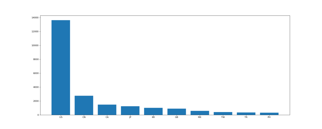
使用matplotlib呈现出店铺总数排名前10的国家
# coding=utf-8
import pandas as pd
from matplotlib import pyplot as plt

file_path = "./starbucks_store_worldwide.csv"

df = pd.read_csv(file_path)

# 使用matplotlib呈现出店铺总数排名前10的国家
# 准备数据
data1 = df.groupby(by="Country").count()["Brand"].sort_values(ascending=False)[:10]

_x = data1.index
_y = data1.values

# 画图
plt.figure(figsize=(20, 8), dpi=80)

plt.bar(range(len(_x)), _y)

plt.xticks(range(len(_x)), _x)

plt.savefig("./t1.png")
使用matplotlib呈现出每个中国每个城市的店铺数量
import pandas as pd
import numpy as np
from matplotlib import pyplot as plt

plt.rcParams['font.sans-serif'] = ['Microsoft YaHei']

file_path = "./starbucks_store_worldwide.csv"

df = pd.read_csv(file_path)
df = df[df["Country"] == "CN"]
print(df.head(1))

# 使用matplotlib呈现出店铺总数排名前10的国家
# 准备数据
data1 = df.groupby(by="City").count()["Brand"].sort_values(ascending=False)[:25]

_x = data1.index
_y = data1.values

# 画图
plt.figure(figsize=(20, 8), dpi=80)

plt.bar(range(len(_x)), _y, width=0.3, color="cyan")

plt.xticks(range(len(_x)), _x)

plt.savefig("./t1.png")
 还记得吗?”卡宴”色!?
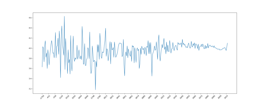
现在我们有全球排名靠前的10000本书的数据,那么请统计一下下面几个问题:
- 不同年份书的数量
- 不同年份书的平均评分情况
import pandas as pd
from matplotlib import pyplot as plt

file_path = "./books.csv"

df = pd.read_csv(file_path)

# 不同年份书的数量
# data1 = df[pd.notna(df["original_publication_year"])]
#
# grouped = data1.groupby(by="original_publication_year").count()["title"]

# 不同年份书的平均评分情况
# 去除original_publication_year列中的nan的行
data1 = df[pd.notnull(df["original_publication_year"])]

grouped = data1["average_rating"].groupby(by=data1["original_publication_year"]).mean()

_x = grouped.index
_y = grouped.values

# 画图
plt.figure(figsize=(20, 8), dpi=80)
plt.plot(range(len(_x)), _y)

plt.xticks(list(range(len(_x)))[::10],_x[::10].astype(int),rotation=45)
plt.savefig("./t1.png")
现在我们有2015到2017年25万条911的紧急电话的数据,请统计出出这些数据中不同类型的紧急情况的次数,如果我们还想统计出不同月份不同类型紧急电话的次数的变化情况,应该怎么做呢?
数据来源:https://www.kaggle.com/mchirico/montcoalert/data
不同类型的紧急情况的次数
import pandas as pd
from matplotlib import pyplot as plt
import numpy as np

df = pd.read_csv("./911.csv")

# 获取分类
# print(df["title"].str.split(": "))
temp_list = df["title"].str.split(": ").tolist()
cate_list = list(set([i[0] for i in temp_list]))
print(cate_list)

# 构造全为0的数组
zeros_df = pd.DataFrame(np.zeros((df.shape[0], len(cate_list))), columns=cate_list)

# 赋值
for cate in cate_list:
    zeros_df[cate][df["title"].str.contains(cate)] = 1

# print(zeros_df)

sum_ret = zeros_df.sum(axis=0)
print(sum_ret)
运行结果
['EMS', 'Fire', 'Traffic']
EMS        124844.0
Fire        37432.0
Traffic     87465.0
dtype: float64
不同月份不同类型紧急电话的次数
import pandas as pd
from matplotlib import pyplot as plt
import numpy as np

df = pd.read_csv("./911.csv")

# 获取分类
# print(df["title"].str.split(": "))
temp_list = df["title"].str.split(": ").tolist()
cate_list = [i[0] for i in temp_list]
df["cate"] = pd.DataFrame(np.array(cate_list).reshape((df.shape[0], 1)))

# print(df.head(5))
print(df.groupby(by="cate").count()["title"])
运行结果
cate
EMS        124840
Fire        37432
Traffic     87465
Name: title, dtype: int64
pandas时间序列
为什么要学习pandas中的时间序列
不管在什么行业,时间序列都是一种非常重要的数据形式,很多统计数据以及数据的规律也都和时间序列有着非常重要的联系
而且在pandas中处理时间序列是非常简单的
生成一段时间范围
pd.date_range(start=None, end=None, periods=None, freq=’D’)
start和end以及freq配合能够生成start和end范围内以频率freq的一组时间索引start和periods以及freq配合能够生成从start开始的频率为freq的periods个时间索引
In [141]: pd.date_range(start = "20170101", end="20170924")
Out[141]:
DatetimeIndex(['2017-01-01', '2017-01-02', '2017-01-03', '2017-01-04',
               '2017-01-05', '2017-01-06', '2017-01-07', '2017-01-08',
               '2017-01-09', '2017-01-10',
               ...
               '2017-09-15', '2017-09-16', '2017-09-17', '2017-09-18',
               '2017-09-19', '2017-09-20', '2017-09-21', '2017-09-22',
               '2017-09-23', '2017-09-24'],
              dtype='datetime64[ns]', length=267, freq='D')

In [142]: pd.date_range(start = "20170101", end="20170924", freq="BM")
Out[142]:
DatetimeIndex(['2017-01-31', '2017-02-28', '2017-03-31', '2017-04-28',
               '2017-05-31', '2017-06-30', '2017-07-31', '2017-08-31'],
              dtype='datetime64[ns]', freq='BM')

In [143]: pd.date_range(start = "20170101", periods=10, freq="WOM-3FRI")
Out[143]:
DatetimeIndex(['2017-01-20', '2017-02-17', '2017-03-17', '2017-04-21',
               '2017-05-19', '2017-06-16', '2017-07-21', '2017-08-18',
               '2017-09-15', '2017-10-20'],
              dtype='datetime64[ns]', freq='WOM-3FRI')
关于频率的更多缩写
| 别名 | 偏移量类型 | 说明 |
|---|---|---|
| D | Day | 每日历日 |
| B | BusinessDay | 每工作日 |
| H | Hour | 每小时 |
| T或min | Minute | 每分 |
| S | Second | 每秒 |
| L或ms | Milli | 每毫秒(即每千分之一秒) |
| U | Micro | 每微秒(即每百万分之-一秒) |
| M | MonthEnd | 每月最后一个日历日 |
| BM | BusinessMonthEnd | 每月最后一个工作日 |
| MS | MonthBegin | 每月第一个日历日 |
| BMS | BusinessMonthBegin | 每月第一个工作日 |
在DataFrame中使用时间序列
index=pd.date_range("20170101",periods=10)
df = pd.DataFrame(np.random.rand(10),index=index)
回到最开始的911数据的案例中,我们可以使用pandas提供的方法把时间字符串转化为时间序列
df["timeStamp"] = pd.to_datetime(df["timeStamp"],format="")
format参数大部分情况下可以不用写,但是对于pandas无法格式化的时间字符串,我们可以使用该参数,比如包含中文
那么问题来了:我们现在要统计每个月或者每个季度的次数怎么办呢?
pandas重采样
重采样:指的是将时间序列从一个频率转化为另一个频率进行处理的过程,将高频率数据转化为低频率数据为降采样,低频率转化为高频率为升采样
pandas提供了一个resample的方法来帮助我们实现频率转化
In [144]: t = pd.DataFrame(np.random.uniform(10, 50, (100, 1)),index=pd.date_range("20170101", periods=100))

In [145]: t
Out[145]:
                    0
2017-01-01  31.152706
2017-01-02  44.722549
2017-01-03  10.334364
2017-01-04  46.476915
2017-01-05  27.987140
2017-01-06  15.970092
2017-01-07  23.283627
2017-01-08  13.868859
2017-01-09  33.449184
2017-01-10  33.290010
2017-01-11  33.945526
2017-01-12  13.973722
2017-01-13  17.000331
2017-01-14  46.062040
2017-01-15  33.769615
2017-01-16  29.393069
2017-01-17  28.017411
2017-01-18  17.243368
2017-01-19  11.243506
2017-01-20  42.693308
2017-01-21  28.940701
2017-01-22  23.727532
2017-01-23  19.294009
2017-01-24  26.742469
2017-01-25  24.595461
2017-01-26  24.175846
2017-01-27  41.257903
2017-01-28  22.319907
2017-01-29  13.972438
2017-01-30  10.084155
...               ...
2017-03-12  32.409551
2017-03-13  27.694186
2017-03-14  22.322692
2017-03-15  23.418212
2017-03-16  15.969703
2017-03-17  31.262390
2017-03-18  35.365964
2017-03-19  26.810274
2017-03-20  41.379748
2017-03-21  29.820417
2017-03-22  34.034580
2017-03-23  45.289687
2017-03-24  47.151367
2017-03-25  26.168448
2017-03-26  36.962455
2017-03-27  43.296036
2017-03-28  42.935293
2017-03-29  27.558675
2017-03-30  43.968883
2017-03-31  11.298828
2017-04-01  37.492047
2017-04-02  48.955097
2017-04-03  36.288276
2017-04-04  10.841008
2017-04-05  28.645696
2017-04-06  37.567298
2017-04-07  17.394214
2017-04-08  41.061697
2017-04-09  10.810684
2017-04-10  18.122624

[100 rows x 1 columns]

In [147]: t.resample("M").mean()
Out[147]:
                    0
2017-01-31  26.358673
2017-02-28  29.803439
2017-03-31  30.990791
2017-04-30  28.717864

In [148]: t.resample("10D").count()
Out[148]:
             0
2017-01-01  10
2017-01-11  10
2017-01-21  10
2017-01-31  10
2017-02-10  10
2017-02-20  10
2017-03-02  10
2017-03-12  10
2017-03-22  10
2017-04-01  10

In [149]: t.resample("QS-JAN").count()
Out[149]:
             0
2017-01-01  90
2017-04-01  10
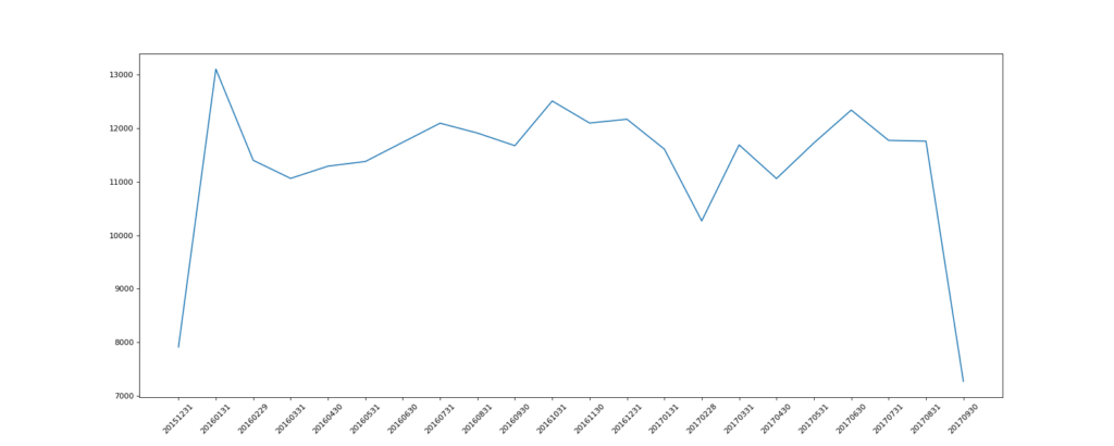
1. 统计出911数据中不同月份电话次数的变化情况
import pandas as pd
from matplotlib import pyplot as plt
import numpy as np

df = pd.read_csv("./911.csv")

df["timeStamp"] = pd.to_datetime(df["timeStamp"])
df.set_index("timeStamp", inplace=True)

print(df.head())

# 统计出911数据中不同月份电话次数的
count_by_month = df.resample("M").count()["title"]
print(count_by_month)

# 画图
_x = count_by_month.index
_y = count_by_month.values

_x = [i.strftime("%Y%m%d") for i in _x]

plt.figure(figsize=(20, 8), dpi=80)

plt.plot(range(len(_x)), _y)
plt.xticks(range(len(_x)), _x, rotation=45)

plt.savefig("./t.png")
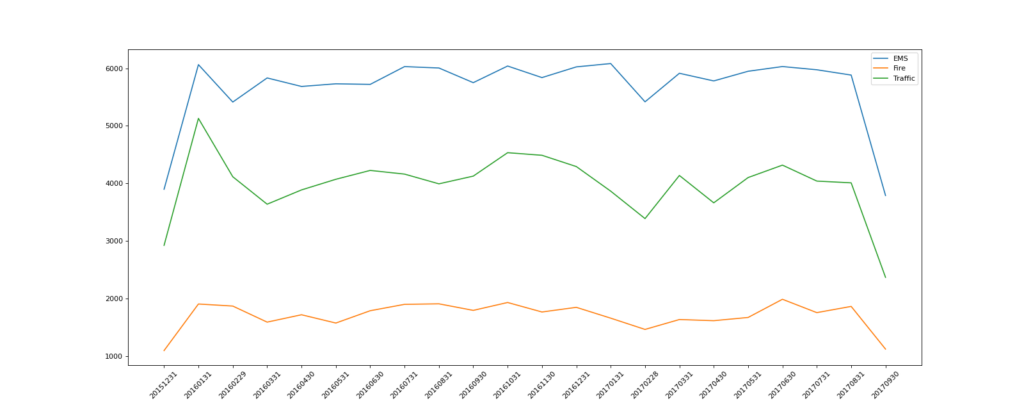
2. 统计出911数据中不同月份不同类型的电话的次数的变化情况
# coding=utf-8
# 911数据中不同月份不同类型的电话的次数的变化情况
import pandas as pd
import numpy as np
from matplotlib import pyplot as plt

# 把时间字符串转为时间类型设置为索引
df = pd.read_csv("./911.csv")
df["timeStamp"] = pd.to_datetime(df["timeStamp"])

# 添加列,表示分类
temp_list = df["title"].str.split(": ").tolist()
cate_list = [i[0] for i in temp_list]
# print(np.array(cate_list).reshape((df.shape[0],1)))
df["cate"] = pd.DataFrame(np.array(cate_list).reshape((df.shape[0], 1)))

df.set_index("timeStamp", inplace=True)

print(df.head(1))

plt.figure(figsize=(20, 8), dpi=80)

# 分组
for group_name, group_data in df.groupby(by="cate"):
    # 对不同的分类都进行绘图
    count_by_month = group_data.resample("M").count()["title"]

    # 画图
    _x = count_by_month.index
    print(_x)
    _y = count_by_month.values

    _x = [i.strftime("%Y%m%d") for i in _x]

    plt.plot(range(len(_x)), _y, label=group_name)

plt.xticks(range(len(_x)), _x, rotation=45)
plt.legend(loc="best")
plt.savefig("./t.png")
现在我们有北上广、深圳、和沈阳5个城市空气质量数据,请绘制出5个城市的PM2.5随时间的变化情况
 数据来源:https://www.kaggle.com/uciml/pm25-data-for-five-chinese-cities
观察这组数据中的时间结构,并不是字符串,这个时候我们应该怎么办?
PeriodIndex
之前所学习的DatetimeIndex可以理解为时间戳那么现在我们要学习的PeriodIndex可以理解为时间段
periods = pd.PeriodIndex(year=data["year"],month=data["month"],day=data["day"],hour=data["hour"],freq="H")
那么如果给这个时间段降采样呢?
data = df.set_index(periods).resample("10D").mean()
绘制中国和美国的的PM2.5随时间的变化情况
# coding=utf-8
import pandas as pd
from matplotlib import pyplot as plt

file_path = "./PM2.5/BeijingPM20100101_20151231.csv"

df = pd.read_csv(file_path)

# 把分开的时间字符串通过periodIndex的方法转化为pandas的时间类型
period = pd.PeriodIndex(year=df["year"], month=df["month"], day=df["day"], hour=df["hour"], freq="H")
df["datetime"] = period
# print(df.head(10))

# 把datetime 设置为索引
df.set_index("datetime", inplace=True)

# 进行降采样
df = df.resample("7D").mean()
print(df.head())
# 处理缺失数据,删除缺失数据
# print(df["PM_US Post"])

data = df["PM_US Post"]
data_china = df["PM_Nongzhanguan"]

print(data_china.head(100))
# 画图
_x = data.index
_x = [i.strftime("%Y%m%d") for i in _x]
_x_china = [i.strftime("%Y%m%d") for i in data_china.index]
print(len(_x_china), len(_x_china))
_y = data.values
_y_china = data_china.values

plt.figure(figsize=(20, 8), dpi=80)

plt.plot(range(len(_x)), _y, label="US_POST", alpha=0.7)
plt.plot(range(len(_x_china)), _y_china, label="CN_POST", alpha=0.7)

plt.xticks(range(0, len(_x_china), 10), list(_x_china)[::10], rotation=45)

plt.legend(loc="best")

plt.savefig('./t.png')
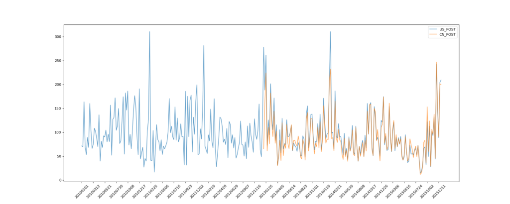
我也好奇China怎么就出来一半,之后我打印了以下数据,China丢了那么一些数据,都是NaN……
               No    year     month  ...        Iws  precipitation     Iprec
datetime                             ...
2010-01-01   84.5  2010.0  1.000000  ...  43.859821       0.066667  0.786905
2010-01-08  252.5  2010.0  1.000000  ...  45.392083       0.000000  0.000000
2010-01-15  420.5  2010.0  1.000000  ...  17.492976       0.000000  0.000000
2010-01-22  588.5  2010.0  1.000000  ...  54.854048       0.000000  0.000000
2010-01-29  756.5  2010.0  1.571429  ...  26.625119       0.000000  0.000000
[5 rows x 17 columns]
datetime
2010-01-01   NaN
2010-01-08   NaN
2010-01-15   NaN
2010-01-22   NaN
2010-01-29   NaN
              ..
2011-10-28   NaN
2011-11-04   NaN
2011-11-11   NaN
2011-11-18   NaN
2011-11-25   NaN
Freq: 7D, Name: PM_Nongzhanguan, Length: 100, dtype: float64
313 313
不过没关系,我们以学习为主。
“坚定选择方向,始终相信爱与善良”
2020-8-18 深夜
Macsen Chu


 1万+
1万+

 被折叠的 条评论
为什么被折叠?
被折叠的 条评论
为什么被折叠?
 到【灌水乐园】发言


