python画卡通_python绘制参数方程的动画

© 2018 *All rights reserved by liudx .:smile:

​ Python的matplotlib是一个功能强大的绘图库，可以很方便的绘制数学图形。官方给出了很多简单的实例，结合中文翻译的示例Tutorial，可以满足日常工作的大部分需求了。但是实际工作中，一些有趣的东西很难使用常规方程（笛卡尔坐标和极坐标）方式绘制，事实上，大部分工程上都是使用参数方程来描述曲线。本文给出一些参数方程绘制的实例，之后会扩展为动画形式绘制，可以看到这些复杂的方程是如何简单优美的绘制出来。

1 参数方程绘制

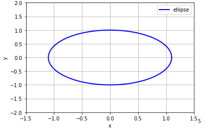
​ 首先介绍下椭圆的参数方程：

$$

begin{cases}

x = a cdot cos(t)\

y = b cdot sin(t)

end{cases}

$$

​ 其中$a,b$分别是椭圆的长轴、短轴。绘制椭圆的python代码如下:

1

2

3

4

5

6

7

8

9

10

11

12

13

14

15

16

17

18import matplotlib.pyplot as plt

import numpy as np

fig = plt.figure()

ax = plt.gca()

r1 = 1.1

r2 = 1

t = np.linspace(0, np.pi*2, 1000) # 生成参数t的数组

x = r1 * np.cos(t)

y = r2 * np.sin(t)

plt.plot(x, y, color='blue', linewidth=2, label='ellipse')

plt.xlabel('x')

plt.ylabel('y')

plt.ylim(-2, 2)

plt.xlim(-1.5,1.5)

ax.grid()

plt.show()

​ 结果如下:

​

​ 下面我们来个复杂点的例子，绘制炮弹的弹道曲线（当然是理想情况的），我们先根据公式推算一把，首先我们设炮弹出口速度$v_0(m/s)$,向上仰角为$theta$ °，时间为$t(s)$, 大炮的筒口初始坐标初始为(0,0)，则有：

$$

begin{cases}

x=v_0cdotsin(theta)cdot t \

y=v_0cdotcos(theta)cdot t - v_0cdotcos(theta)cdot g cdot t^2

end{cases}

$$

​ 对应python代码為：

1

2

3

4

5

6

7

8

9

10

11

12

13

14

15

16

17

18

19

20

21

22

23

24

25

26def (v0, theta_x): # 模拟炮弹飞行曲线

g = 9.80665 # m/s^2

v0_x = v0*np.cos(theta_x)

v0_y = v0*np.sin(theta_x)

t_m = (v0_y / g) # 飞行时间

#h = g*t_m**2/2

t = np.linspace(0, v0_x * t_m * 2, v0*1000)

x = v0_x * t

y = v0_y *t - v0_y *g * t**2 / 2

return x,y

if __name__ == '__main__':

linestyles = ['-', '--', '-.', ':']

x1, y1 = Parabolic(100, np.deg2rad(45))

x2, y2 = Parabolic(100, np.deg2rad(30))

x3, y3 = Parabolic(100, np.deg2rad(60))

plt.plot(x1, y1, color='r', linewidth=1, linestyle="--",label='45deg')

plt.plot(x2, y2, color='y', linewidth=1, linestyle="-.", label='30deg')

plt.plot(x3, y3, color='c', linewidth=1, linestyle=":", label='60deg')

plt.xlabel('x')

plt.ylabel('h')

plt.xlim(0, 20)

plt.ylim(0, 8)

plt.legend(loc='upper center')

plt.show()

​ 为了方便示意，我分别绘制了初速为$100m/s$时，仰角为45°、30°、60°的炮弹落地曲线：

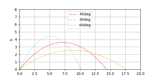
​ 验证了我们高中物理中的一个结论：这货不就是抛物线嘛。

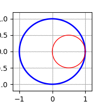
​ 看完静态的参数方程，还是不过瘾，我们来做个动画玩玩。首先是绘制一个内旋轮，引用下这位老哥的例子：

1

2

3

4

5

6

7

8

9

10

11

12

13

14

15

16

17

18

19

20

21

22

23

24

25

26

27

28

29

30import numpy as np

import matplotlib

import matplotlib.pyplot as plt

import matplotlib.animation as animation

fig = plt.figure(figsize=(6, 6)) # 图像大小

ax = plt.gca()

ax.grid()

ln1, = ax.plot([], [], '-', color='b', lw=2) # 注意逗号，取出plot数据:plot return A list of Line2D objects representing the plotted data.

ln2, = ax.plot([], [], '-', color='r', lw=1)

theta = np.linspace(0, 2*np.pi, 100) # 参数t的数组

r_out = 1 # 静态圆的半径

r_in = 0.5 # 动态圆的半径

def init():

ax.set_xlim(-2, 2)

ax.set_ylim(-2, 2)

x_out = [r_out*np.cos(theta[i]) for i in range(len(theta))]

y_out = [r_out*np.sin(theta[i]) for i in range(len(theta))]

ln1.set_data(x_out, y_out) # 静圆

return ln1, # 此处返回tuple

def update(i): # 每次回调时，传入索引`0~range(len(theta))`,注意repeat时索引会归0

x_in = [(r_out-r_in)*np.cos(theta[i])+r_in*np.cos(theta[j]) for j in range(len(theta))]

y_in = [(r_out-r_in)*np.sin(theta[i])+r_in*np.sin(theta[j]) for j in range(len(theta))]

ln2.set_data(x_in, y_in) # 动圆

return ln2,

ani = animation.FuncAnimation(fig, update, range(len(theta)), init_func=init, interval=30)

#ani.save('roll.gif', writer='imagemagick', fps=100)

plt.show()

​ 看起来很不错，能动(这里发现了init函数可以绘制下静态的大圆ln1，update函数只对动圆ln2的plot对象数据进行更新)：

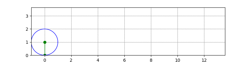
​ 最后研究下旋轮线, 看看能否绘制出wiki页面上那个动画效果。先列出参数方程：

$$

选轮线参数方程：

begin{cases}

x = rcdot(t-sin t) \

y = r cdot (1-cos t)

end{cases}

\

圆心的坐标为:(t,r)

$$

​ 经过观察摸索，发现需要绘制3部分，一个是滚动的圆，一个是摆线，还有个圆心到绘制曲线的支点。坐标都可直接从参数方程推算出来，不多说，直接上代码和注释吧：

1

2

3

4

5

6

7

8

9

10

11

12

13

14

15

16

17

18

19

20

21

22

23

24

25

26

27

28

29

30

31

32

33

34

35

36

37

38

39

40

41

42

43#def wheel_line():

fig = plt.figure(figsize=(8,2))

ax = plt.gca()

ax.grid()

ln, = ax.plot([], [], 'o-', color='g', lw=1) # 圆心连线 @center -> curve

circle, = ax.plot([], [], '-', color='b', lw=1) # 滚动的圆

curve, = ax.plot([], [], '-', color='r', lw=1) # 摆线

curve_x, curve_y = [], []

r = 1

t = np.linspace(0, math.pi*2, 1000)

L = 4*np.pi*r

theta = np.linspace(0, L, 250)

def init():

ax.set_xlim(-r, L + r)

ax.set_ylim(0, L/4 + r/2)

ln.set_data([0,0], [0,1])

x_out = r*np.cos(t)

y_out = r*np.sin(t) + r

circle.set_data(x_out, y_out)

return circle,ln

def update(frame):

tt = theta[frame] # 获取参数t

x=r*(tt-np.sin(tt))

y=r*(1-np.cos(tt))

curve_x.append(x)

curve_y.append(y)

curve.set_data(curve_x, curve_y) # 更新摆线

if i == len(theta) - 1:

curve_x.clear()

curve_y.clear()

# update circle

x_out = r*np.cos(t) + tt

y_out = r*np.sin(t) + r

circle.set_data(x_out, y_out)

# new circle center @(tt,r)

ln.set_data([tt,x],[r,y])

return curve,circle,ln

ani = animation.FuncAnimation(fig, update, frames=range(len(theta)), init_func=init, interval=1)

ani.save('roll.gif', writer='imagemagick', fps=60)

plt.show()

​ 大功告成:

3 后记

​ 在摸索过程中，还是有很多坑需要注意的，最初那个摆线的例子，我没有计算好图形范围，画出来的圆是扁扁的，后来通过改figsize和ax.set_xlim/set_ylim为相同比例解决的；保存动画那个ani.save('roll.gif', writer='imagemagick', fps=60)总是报错，经过查找资料，解决方案是安装imagemagic，下载安装后第2节的例子都能顺利保存动图为gif。还有需要注意是的save函数里面的fps参数不能调太低，否则会出现动画卡顿的现象，太高又会出现动画速度很快的问题，这个参数需要配合frames即动画的总帧数，以及FuncAnimation里面的interval帧间隔时间参数(单位是ms)，总动画时间(秒)公式为：$frames * interval/1000+frames/fps$。

​ 读完这篇文章，相信绘制参数方程和动画不是一件难事吧:smile:。