逻辑回归（Logistic Regression）及在spark,sklearn等的应用（更新ing）

参考Logistics Regression
参考 李航.统计学习方法[M].清华大学出版社

概述

• 本质上是一个分类模型，常用于二分类
• 本质： 假设数据服从这个分布，然后使用极大似然估计做参数的估计

Logistic分布

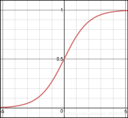
logistic 分布是一种连续型的分布，其分布函数和密度函数分别为：

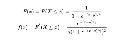
u 表示位置参数，$$r$$>0 为形状参数。 logistic 分布是由其位置参数和尺度参数 定义的连续分布。其分布的形状与正态分布形状相似，但其尾部更长。

逻辑回归和线性回归比较

线性回归预测输出的是连续值
线性表达式：
$$f(x)=w^{t}x+b$$
为了消除掉后面的常数项b，我们可以令 $$x^{\prime }={\left[\begin{array}{ll}1& x\end{array}\right]}^T$$ ，同时$$w^{\prime }={\left[\begin{array}{ll}b& w\end{array}\right]}^T$$ ，也就是说给x多加一项而且值恒为1，这样b就到了w里面去了，直线方程可以化简成为

$$f\left({\mathbf{x}}^{\prime }\right)={\mathbf{w}}^{\prime T}{\mathbf{x}}^{\prime }$$
逻辑回归输出的是离散的值
分为二分类和多分类
为了得到预测概率值。我们用sigmoid激活函数。
$$g(z)=\frac{1}{1+e^{-z}}$$
g(𝑧) in [0,1]
$z=w^{t}x+b$

逻辑回归模型

$$h_{\theta }(x)={\theta }_0+{\theta }_1{x}_1+{\theta }_2{x}_2+\cdots +{\theta }_n{x}_n$$
逻辑回归的假设函数可以表示为
$$h_{\theta }(x)=\mathrm{g}\left({\theta }^{T}x\right)$$$$g(z)=\frac{1}{1+e^{-z}}$$
即$$\begin{array}{l}y=1\to {\theta }^{\mathrm{T}}x\ge 0\\ y=0\to {\theta }^{\mathrm{T}}x<0\end{array}$$
注意
$$g(z)=\frac{1}{1+e^{-z}}=\frac{e^z}{1+e^z}$$
$$g(-z)=1-\frac{1}{1+e^{-z}}=\frac{1}{1+e^z}$$

二项逻辑回归模型是如下的条件概率分布：

$$\mathrm{P}(\mathrm{y}=1|\mathrm{x},\theta )=\frac{1}{1+e^{-{\theta }^{T}x}}=\frac{e^{{\theta }^{T}x}}{1+e^{{\theta }^{T}x}}$$$$\mathrm{p}(\mathrm{y}=0|\mathrm{x},\theta )=\frac{1}{1+e^{-{\theta }^{T}x}}=1-p(\mathrm{y}=1|\mathrm{x},\theta )=\mathrm{p}(\mathrm{y}=1|\mathrm{x},-\theta )=\frac{1}{1+e^{{\theta }^{T}x}}$$

pyspark 应用

• 定义

class pyspark.ml.classification.LogisticRegression(featuresCol='features', labelCol='label', predictionCol='prediction', maxIter=100, regParam=0.0, elasticNetParam=0.0, tol=1e-06, fitIntercept=True, threshold=0.5, thresholds=None, probabilityCol='probability', rawPredictionCol='rawPrediction', standardization=True, weightCol=None, aggregationDepth=2, family='auto', lowerBoundsOnCoefficients=None, upperBoundsOnCoefficients=None, lowerBoundsOnIntercepts=None, upperBoundsOnIntercepts=None)

• 官方demo

bdf = spark.createDataFrame([
    Row(label=1.0, weight=1.0, features=Vectors.dense(0.0, 5.0)),
    Row(label=0.0, weight=2.0, features=Vectors.dense(1.0, 2.0)),
    Row(label=1.0, weight=3.0, features=Vectors.dense(2.0, 1.0)),
    Row(label=0.0, weight=4.0, features=Vectors.dense(3.0, 3.0))])

blor = LogisticRegression(regParam=0.01, weightCol="weight",rawPredictionCol='rawPrediction')
blorModel = blor.fit(bdf)

# print(type(blorModel)) #<class 'pyspark.ml.classification.LogisticRegressionModel'>
# print(dir(blorModel))
print(blorModel.coefficients)

test0=spark.createDataFrame([Row(features=Vectors.dense(-1.,1.))])
result=blorModel.transform(test0)
result.show()
"""
+----------+--------------------+--------------------+----------+
|  features|       rawPrediction|         probability|prediction|
+----------+--------------------+--------------------+----------+
|[-1.0,1.0]|[-3.5472025573965...|[0.02799860485691...|       1.0|
+----------+--------------------+--------------------+----------+
"""

# print(dir(result))
print(result.select('probability').take(1))
print(result.select('rawPrediction').take(1))
# [Row(probability=DenseVector([0.028, 0.972]))]
# [Row(rawPrediction=DenseVector([-3.5472, 3.5472]))]

• 释义
  如果是二分类
  rawPrediction 等同于wx + b
  pbobability 等同于1/(1+e^-(wx + b))
  prediction 为0 或1
• 参数解释
  featuresCol=“features”: 输入训练集和预测数据集中的属性向量的字段名称
  labelCol=“label”: 输入训练集集中的标记字段
  predictionCol=“prediction”: 输出结果中判别字段名称
  maxIter=100: 迭代算法的最大迭代次数
  regParam=0.0: 正则化惩罚程度参数
  elasticNetParam=0.0: 正则化时弹性网络调整参数
  tol=1e-6:收敛容忍系数(convergence tolerance)，算法每次迭代后的比较阈值来确定算法是否结束，值越小，可能执行的迭代次数就越多。
  fitIntercept=True: 是否使用带截距的回归
  threshold=0.5:
  thresholds=None:
  probabilityCol=“probability”, 输出结果概率值名称
  rawPredictionCol=“rawPrediction” ：输出结果数据中回归因变量值的字段名称
  standardization=True:是否在回归前对训练集中的属性数据做标准化处理
  weightCol=None: 权重
  aggregationDepth=2:Spark迭代计算过程中才用treeAggregate的方式来reduce各个分区数据，这里的参数可以用来调整treeAggregate的层次深度，层次越深reduce时用到的执行节点更多，能并行的数据量就越多。(>=2的整数，默认值2)
  family=“auto”:
  可选项
  1 binomial 二分类
  2 multinomial 多分类
  3 auto 自动选择
  lowerBoundsOnCoefficients=None：
  系数的下限约束，能够支持设置多分类(矩阵中每个向量代表一个分类系数)的系数。(矩阵类型，无默认值)
  upperBoundsOnCoefficients=None：系数的上限约束，能够支持设置多分类(矩阵中每个向量代表一个分类系数)的系数。(矩阵类型，无默认值)
  lowerBoundsOnIntercepts=None： 常量系数(截距)的下限约束，能够支持设置多分类(向量中每个分量代表一个分类系数)的截距。(向量类型，无默认值)upperBoundsOnIntercepts=None:常量系数(截距)的上限约束，能够支持设置多分类(向量中每个分量代表一个分类系数)的截距。(向量类型，无默认值)

sklearn 应用