【python数据分析】：数据建模之线性回归

线性回归通常是人们在学习预测模型时首选的技术之一。

在这种技术中，因变量是连续的，自变量可以是连续的也可以是离散的，回归线的性质是线性的。

线性回归使用最佳的拟合直线（也就是回归线）在因变量（Y）和一个或多个自变量（X）之间建立一种关系。

线性回归：

简单线性回归 / 多元线性回归 /模型评估

简单线性回归（一元线性回归）

# 导入线性回归模块from sklearn.linear_model import LinearRegression

# np.random.RandomState → 随机数种子，对于一个随机数发生器，只要该种子（seed）相同，产生的随机数序列就是相同的# 生成随机数据x与y# 样本关系：y = 8 + 4*xrng = np.random.RandomState(1)  print(rng)xtrain = 10 * rng.rand(30)ytrain = 8 + 4 * xtrain + rng.rand(30)

# 生成散点图fig = plt.figure(figsize =(18,6))ax1 = fig.add_subplot(1,2,1)plt.scatter(xtrain,ytrain,marker = '.',color = 'k')plt.grid()plt.title('样本数据散点图')
# LinearRegression → 线性回归评估器，用于拟合数据得到拟合直线# model.fit(x,y) → 拟合直线，参数分别为x与y# x[:,np.newaxis] → 将数组变成(n,1)形状model = LinearRegression()model.fit(xtrain[:,np.newaxis],ytrain)
# 创建测试数据xtest，并根据拟合曲线求出ytest# model.predict → 预测xtest = np.linspace(0,10,1000)ytest = model.predict(xtest[:,np.newaxis])
# 绘制散点图、线性回归拟合直线ax2 = fig.add_subplot(1,2,2)plt.scatter(xtrain,ytrain,marker = '.',color = 'k')plt.plot(xtest,ytest,color = 'r')plt.grid()plt.title('线性回归拟合')

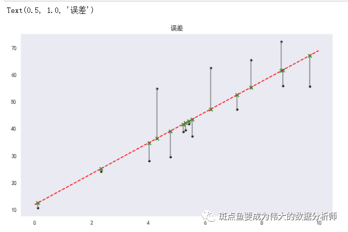
# 误差可视化
rng = np.random.RandomState(8)xtrain = 10 * rng.rand(15)ytrain = 8 + 4 * xtrain + rng.rand(15) * 30model.fit(xtrain[:,np.newaxis],ytrain)xtest = np.linspace(0,10,1000)ytest = model.predict(xtest[:,np.newaxis])# 创建样本数据并进行拟合fig = plt.figure(figsize =(10,6))plt.plot(xtest,ytest,color = 'r',linestyle = '--')  # 拟合直线plt.scatter(xtrain,ytrain,marker = '.',color = 'k')  # 样本数据散点图ytest2 = model.predict(xtrain[:,np.newaxis])  # 样本数据x在拟合直线上的y值plt.scatter(xtrain,ytest2,marker = 'x',color = 'g')   # ytest2散点图plt.plot([xtrain,xtrain],[ytrain,ytest2],color = 'gray')  # 误差线plt.grid()plt.title('误差')

多元线性回归

​​​​​​​

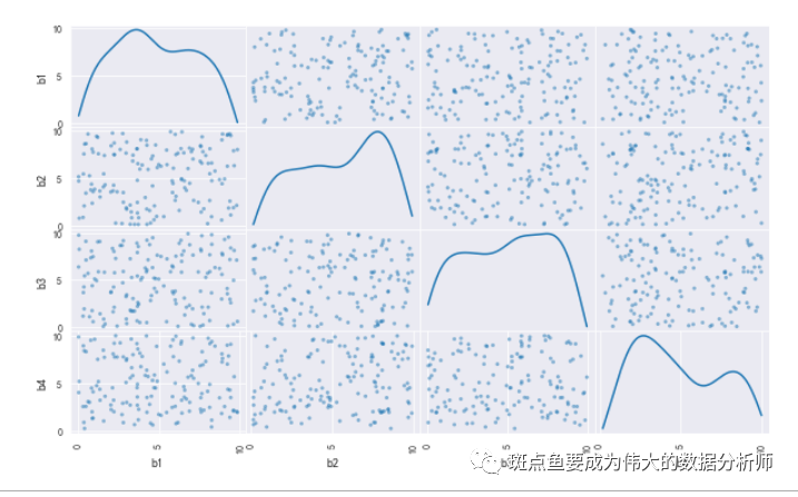
## 创建数据，其中包括4个自变量# 4个变量相互独立rng = np.random.RandomState(5)  xtrain = 10 * rng.rand(150,4)ytrain = 20 + np.dot(xtrain ,[1.5,2,-4,3])df = pd.DataFrame(xtrain, columns = ['b1','b2','b3','b4'])df['y'] = ytrain

pd.plotting.scatter_matrix(df[['b1','b2','b3','b4']],figsize=(10,6),                 diagonal='kde',                 alpha = 0.5,                 range_padding=0.1)print(df.head())
# 多元回归拟合model = LinearRegression()model.fit(df[['b1','b2','b3','b4']],df['y'])
# 参数输出print('斜率a为：' ,model.coef_)print('截距b为：%.4f' % model.intercept_)print('线性回归函数为：\ny = %.1fx1 + %.1fx2 + %.1fx3 + %.1fx4 + %.1f'       % (model.coef_[0],model.coef_[1],model.coef_[2],model.coef_[3],model.intercept_))

 b1        b2        b3        b4          y
0  2.219932  8.707323  2.067192  9.186109  60.034105
1  4.884112  6.117439  7.659079  5.184180  24.477270
2  2.968005  1.877212  0.807413  7.384403  47.129990
3  4.413092  1.583099  8.799370  2.740865   2.810948
4  4.142350  2.960799  6.287879  5.798378  24.378742
斜率a为：[ 1.5  2.  -4.   3. ]
截距b为：20.0000
线性回归函数为：
y = 1.5x1 + 2.0x2 + -4.0x3 + 3.0x4 + 20.0

线性回归模型评估

SSE(和方差、误差平方和)：The sum of squares due to error

MSE(均方差、方差)：Mean squared error

RMSE(均方根、标准差)：Root mean squared error

R-square(确定系数) Coefficient of determination

from sklearn import metrics
rng = np.random.RandomState(1)  xtrain = 10 * rng.rand(30)ytrain = 8 + 4 * xtrain + rng.rand(30) * 3# 创建数据
model = LinearRegression()model.fit(xtrain[:,np.newaxis],ytrain)# 多元回归拟合
ytest = model.predict(xtrain[:,np.newaxis])  # 求出预测数据mse = metrics.mean_squared_error(ytrain,ytest)  # 求出均方差rmse = np.sqrt(mse)  # 求出均方根
#ssr = ((ytest - ytrain.mean())**2).sum()  # 求出预测数据与原始数据均值之差的平方和#sst = ((ytrain - ytrain.mean())**2).sum()  # 求出原始数据和均值之差的平方和#r2 = ssr / sst # 求出确定系数
r2 = model.score(xtrain[:,np.newaxis],ytrain)  # 求出确定系数print("均方差MSE为: %.5f" % mse)print("均方根RMSE为: %.5f" % rmse)print("确定系数R-square为: %.5f" % r2)# 确定系数R-square非常接近于1，线性回归模型拟合较好

均方差MSE为: 0.78471
均方根RMSE为: 0.88584
确定系数R-square为: 0.99465