Pytorch深度学习框架60天进阶学习计划 - 第55天：3D视觉基础（一）

Pytorch深度学习框架60天进阶学习计划 - 第55天：3D视觉基础（一）

今天我们将踏入3D视觉的精彩领域，深入研究点云特征提取网络，对比不同的处理方法，并推导旋转等变卷积的数学原理。系好安全带，我们要开始一段从点到面、从静态到动态的3D视觉之旅了！*

第一部分：点云特征提取基础与方法对比

1. 3D点云数据表示与挑战

3D点云是表示三维物体或场景最原始、最直接的方式之一。它由一系列点组成，每个点都有其在3D空间中的坐标，通常表示为 (x, y, z)，有些还包含颜色、反射强度等额外属性。

点云数据通常来源于：

• 激光雷达 (LiDAR) 扫描
• RGB-D相机(如Kinect)
• 多视角立体重建
• 计算机辅助设计(CAD)模型转换

1.1 点云数据的特性与挑战

处理点云数据面临几个独特的挑战：

特性	描述	挑战
无序性	点云中的点没有固定顺序	需要设计排列不变的算法
不规则性	点分布不均匀，密度可变	难以应用传统的卷积操作
刚性变换	旋转、平移不应改变物体识别结果	需要旋转平移不变性
规模多变	点数量从数百到数百万不等	计算复杂度难以控制
局部结构	点与近邻点构成局部几何结构	需有效捕获局部特征

1.2 点云处理方法的分类

针对这些挑战，研究者提出了多种处理方法，大致可分为三类：

1. 体素化方法：将点云转换为规则的3D网格
2. 原始点云方法：直接处理无序点集
3. 混合方法：结合体素和原始点云的优势
   

2. 体素化方法详解

体素化(Voxelization)是将不规则的点云转换为规则3D网格的过程，类似于将2D图像像素化。

2.1 体素化的基本原理

体素化的基本流程如下：

1. 确定体素化范围和分辨率
2. 将3D空间划分为规则网格(体素)
3. 对每个体素，统计落入其中的点的某种特征(如点数、平均值等)
4. 生成结构化的3D体素网格

2.2 代表性体素化网络：VoxNet

VoxNet是最早的体素化深度学习方法之一，它使用3D卷积神经网络处理体素化点云。

import torch
import torch.nn as nn
import torch.nn.functional as F

class VoxNet(nn.Module):
    def __init__(self, num_classes=10, input_size=32):
        super(VoxNet, self).__init__()
        
        # 3D卷积层
        self.conv1 = nn.Conv3d(1, 32, kernel_size=5, stride=2)
        self.bn1 = nn.BatchNorm3d(32)
        self.conv2 = nn.Conv3d(32, 64, kernel_size=3, stride=1)
        self.bn2 = nn.BatchNorm3d(64)
        
        # 根据输入大小和卷积参数计算全连接层输入尺寸
        # 对于32^3输入，经过第一个卷积层(k=5,s=2)后变为14^3
        # 经过第二个卷积层(k=3,s=1)后变为12^3
        fc_size = 64 * 12 * 12 * 12 if input_size == 32 else 64 * 6 * 6 * 6
        
        # 全连接层
        self.fc1 = nn.Linear(fc_size, 128)
        self.fc2 = nn.Linear(128, num_classes)
        
    def forward(self, x):
        # 输入 x 的形状: [batch_size, 1, D, H, W]
        
        # 3D卷积层 1
        x = F.relu(self.bn1(self.conv1(x)))
        
        # 3D卷积层 2
        x = F.relu(self.bn2(self.conv2(x)))
        
        # 展平
        x = x.view(x.size(0), -1)
        
        # 全连接层
        x = F.relu(self.fc1(x))
        x = F.dropout(x, p=0.5, training=self.training)
        x = self.fc2(x)
        
        return x

# 创建模型实例
model = VoxNet(num_classes=10, input_size=32)

# 测试前向传播
batch_size = 2
voxel_data = torch.rand(batch_size, 1, 32, 32, 32)  # 随机生成32^3的体素数据
output = model(voxel_data)
print(f"Input shape: {voxel_data.shape}")
print(f"Output shape: {output.shape}")

2.3 点云体素化实现

下面是一个将点云转换为体素网格的简单实现：

import numpy as np
import torch
import matplotlib.pyplot as plt
from mpl_toolkits.mplot3d import Axes3D

def voxelize_point_cloud(points, voxel_size=1.0, grid_size=(32, 32, 32)):
    """
    将点云转换为体素网格
    
    参数:
    - points: Nx3 的numpy数组，表示点云
    - voxel_size: 体素的边长
    - grid_size: 网格尺寸 (D, H, W)
    
    返回:
    - voxel_grid: 3D体素网格，形状为grid_size
    """
    # 初始化空体素网格
    voxel_grid = np.zeros(grid_size, dtype=np.float32)
    
    # 计算点云的边界框
    min_bound = np.min(points, axis=0)
    max_bound = np.max(points, axis=0)
    
    # 确保边界框至少与网格一样大
    diff = max_bound - min_bound
    max_diff = np.max(diff)
    if max_diff < voxel_size * max(grid_size):
        # 扩大边界框
        center = (min_bound + max_bound) / 2
        min_bound = center - max(grid_size) * voxel_size / 2
        max_bound = center + max(grid_size) * voxel_size / 2
    
    # 将每个点映射到体素
    grid_indices = np.floor((points - min_bound) / voxel_size).astype(int)
    
    # 过滤出在网格范围内的点
    valid_indices = np.all((grid_indices >= 0) & 
                           (grid_indices < np.array(grid_size)), axis=1)
    valid_grid_indices = grid_indices[valid_indices]
    
    # 统计每个体素中的点数
    for idx in valid_grid_indices:
        x, y, z = idx
        voxel_grid[x, y, z] += 1
    
    # 归一化体素值
    if np.max(voxel_grid) > 0:
        voxel_grid = voxel_grid / np.max(voxel_grid)
    
    return voxel_grid, min_bound, max_bound

# 生成一个简单的球形点云作为示例
def generate_sphere_point_cloud(num_points=1000, radius=1.0, noise=0.05):
    # 随机生成球面上的点
    theta = np.random.uniform(0, 2*np.pi, num_points)
    phi = np.random.uniform(0, np.pi, num_points)
    
    x = radius * np.sin(phi) * np.cos(theta)
    y = radius * np.sin(phi) * np.sin(theta)
    z = radius * np.cos(phi)
    
    points = np.stack([x, y, z], axis=1)
    
    # 添加一些噪声
    noise_vector = np.random.normal(0, noise, points.shape)
    points = points + noise_vector
    
    return points

# 生成点云样本
sphere_points = generate_sphere_point_cloud(num_points=2000, radius=10.0)

# 体素化点云
voxel_size = 1.0
grid_size = (32, 32, 32)
voxel_grid, min_bound, max_bound = voxelize_point_cloud(sphere_points, voxel_size, grid_size)

# 将体素网格转换为PyTorch张量，用于模型输入
voxel_tensor = torch.from_numpy(voxel_grid).float().unsqueeze(0).unsqueeze(0)  # [1, 1, 32, 32, 32]

# 可视化原始点云和体素化结果
fig = plt.figure(figsize=(15, 7))

# 原始点云
ax1 = fig.add_subplot(121, projection='3d')
ax1.scatter(sphere_points[:, 0], sphere_points[:, 1], sphere_points[:, 2], c='b', s=1)
ax1.set_title('原始点云')
ax1.set_xlabel('X轴')
ax1.set_ylabel('Y轴')
ax1.set_zlabel('Z轴')
ax1.set_xlim(min_bound[0], max_bound[0])
ax1.set_ylim(min_bound[1], max_bound[1])
ax1.set_zlim(min_bound[2], max_bound[2])

# 体素化结果（只显示非零体素）
ax2 = fig.add_subplot(122, projection='3d')
voxel_positions = np.where(voxel_grid > 0)
values = voxel_grid[voxel_positions]
ax2.scatter(voxel_positions[0], voxel_positions[1], voxel_positions[2], 
            c=values, cmap='viridis', s=100*values)
ax2.set_title('体素化结果')
ax2.set_xlabel('X轴')
ax2.set_ylabel('Y轴')
ax2.set_zlabel('Z轴')

plt.tight_layout()
plt.savefig('voxelization_visualization.png')
print("可视化结果已保存为'voxelization_visualization.png'")

2.4 体素化方法的优缺点

优点：

• 规则的数据结构，适合传统卷积操作
• 可以直接应用3D卷积神经网络
• 体素之间的空间关系明确

缺点：

• 计算和内存需求随分辨率立方增长（维度灾难）
• 高分辨率下信息损失少但计算昂贵
• 低分辨率下计算高效但信息损失大
• 大量体素可能是空的（稀疏性问题）

2.5 稀疏体素网络

为了解决常规体素化的计算和内存问题，研究者提出了稀疏体素网络，如SparseConvNet和MinkowskiNet，它们只处理非空体素。

# 稀疏体素卷积示例代码（使用MinkowskiEngine库）
import torch
import MinkowskiEngine as ME

class SparseVoxelNet(torch.nn.Module):
    def __init__(self, in_channels=1, out_channels=10):
        super(SparseVoxelNet, self).__init__()
        
        self.conv1 = ME.MinkowskiConvolution(
            in_channels=in_channels,
            out_channels=32,
            kernel_size=3,
            stride=1,
            dimension=3)
            
        self.bn1 = ME.MinkowskiBatchNorm(32)
        self.conv2 = ME.MinkowskiConvolution(
            in_channels=32,
            out_channels=64,
            kernel_size=3,
            stride=2,
            dimension=3)
            
        self.bn2 = ME.MinkowskiBatchNorm(64)
        self.pooling = ME.MinkowskiGlobalPooling()
        self.linear = torch.nn.Linear(64, out_channels)
        
    def forward(self, x):
        # x是一个SparseTensor
        out = self.conv1(x)
        out = self.bn1(out)
        out = ME.MinkowskiReLU()(out)
        
        out = self.conv2(out)
        out = self.bn2(out)
        out = ME.MinkowskiReLU()(out)
        
        # 全局池化得到特征向量
        out = self.pooling(out)
        return self.linear(out)

def points_to_sparse_voxels(points, features=None, voxel_size=1.0):
    """
    将点云转换为稀疏体素格式（适用于MinkowskiEngine）
    
    参数:
    - points: Nx3 的numpy数组，表示点云坐标
    - features: Nx1 的numpy数组，表示每个点的特征（如果为None，则使用全1特征）
    - voxel_size: 体素大小
    
    返回:
    - sparse_tensor: ME.SparseTensor，稀疏体素表示
    """
    if features is None:
        features = np.ones((points.shape[0], 1), dtype=np.float32)
    
    # 量化点坐标
    quantized_points = np.floor(points / voxel_size).astype(np.int32)
    
    # 创建稀疏张量
    coords = torch.from_numpy(quantized_points)
    feats = torch.from_numpy(features)
    
    return ME.SparseTensor(
        features=feats,
        coordinates=ME.utils.batched_coordinates([coords]),
    )

# 注意：以上代码需要安装MinkowskiEngine库才能运行
# pip install -U MinkowskiEngine

3. 原始点云处理方法

与体素化方法不同，原始点云处理方法直接在无序点集上操作，不需要转换为规则网格。

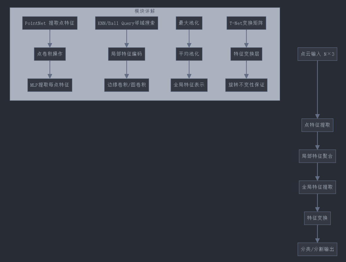
3.1 PointNet：直接处理点云的先驱

PointNet是第一个成功直接处理原始点云的深度学习架构，它具有以下特点：

• 使用逐点MLP (Multi-Layer Perceptron) 提取每个点的特征
• 使用全局最大池化保证排列不变性
• 使用T-Net实现仿射变换不变性

下面是PointNet的基本实现：

import torch
import torch.nn as nn
import torch.nn.functional as F

class TNet(nn.Module):
    """
    T-Net学习仿射变换矩阵，用于输入点云的对齐
    """
    def __init__(self, k=3):
        super(TNet, self).__init__()
        self.k = k
        
        # 共享MLP
        self.conv1 = nn.Conv1d(k, 64, 1)
        self.conv2 = nn.Conv1d(64, 128, 1)
        self.conv3 = nn.Conv1d(128, 1024, 1)
        
        # 全连接层
        self.fc1 = nn.Linear(1024, 512)
        self.fc2 = nn.Linear(512, 256)
        self.fc3 = nn.Linear(256, k*k)
        
        # 批归一化层
        self.bn1 = nn.BatchNorm1d(64)
        self.bn2 = nn.BatchNorm1d(128)
        self.bn3 = nn.BatchNorm1d(1024)
        self.bn4 = nn.BatchNorm1d(512)
        self.bn5 = nn.BatchNorm1d(256)
        
    def forward(self, x):
        batch_size = x.size()[0]
        
        # 应用MLPs (nx3 -> nx64 -> nx128 -> nx1024)
        x = F.relu(self.bn1(self.conv1(x)))
        x = F.relu(self.bn2(self.conv2(x)))
        x = F.relu(self.bn3(self.conv3(x)))
        
        # 全局最大池化
        x = torch.max(x, 2, keepdim=True)[0]
        x = x.view(-1, 1024)
        
        # 全连接层
        x = F.relu(self.bn4(self.fc1(x)))
        x = F.relu(self.bn5(self.fc2(x)))
        x = self.fc3(x)
        
        # 将输出重塑为变换矩阵
        iden = torch.eye(self.k, dtype=x.dtype, device=x.device).view(1, self.k*self.k).repeat(batch_size, 1)
        x = x + iden
        x = x.view(-1, self.k, self.k)
        
        return x

class PointNetBase(nn.Module):
    """
    PointNet基础架构：对点云进行分类
    """
    def __init__(self, num_classes=10, input_transform=True, feature_transform=True):
        super(PointNetBase, self).__init__()
        self.input_transform = input_transform
        self.feature_transform = feature_transform
        
        # 输入变换网络(3x3)
        if self.input_transform:
            self.stn = TNet(k=3)
        
        # 特征提取
        self.conv1 = nn.Conv1d(3, 64, 1)
        self.conv2 = nn.Conv1d(64, 64, 1)
        self.bn1 = nn.BatchNorm1d(64)
        self.bn2 = nn.BatchNorm1d(64)
        
        # 特征变换网络(64x64)
        if self.feature_transform:
            self.fstn = TNet(k=64)
        
        # 更深层特征提取
        self.conv3 = nn.Conv1d(64, 64, 1)
        self.conv4 = nn.Conv1d(64, 128, 1)
        self.conv5 = nn.Conv1d(128, 1024, 1)
        self.bn3 = nn.BatchNorm1d(64)
        self.bn4 = nn.BatchNorm1d(128)
        self.bn5 = nn.BatchNorm1d(1024)
        
        # 分类器
        self.fc1 = nn.Linear(1024, 512)
        self.fc2 = nn.Linear(512, 256)
        self.fc3 = nn.Linear(256, num_classes)
        self.bn6 = nn.BatchNorm1d(512)
        self.bn7 = nn.BatchNorm1d(256)
        self.dropout = nn.Dropout(p=0.3)
        
    def forward(self, x):
        # x的形状: [batch_size, 3, num_points]
        n_pts = x.size()[2]
        
        # 应用输入变换
        if self.input_transform:
            trans = self.stn(x)
            x = torch.bmm(x.transpose(2, 1), trans).transpose(2, 1)
        
        # MLP提取点特征
        x = F.relu(self.bn1(self.conv1(x)))
        x = F.relu(self.bn2(self.conv2(x)))
        
        # 应用特征变换
        if self.feature_transform:
            trans_feat = self.fstn(x)
            x = torch.bmm(x.transpose(2, 1), trans_feat).transpose(2, 1)
        else:
            trans_feat = None
        
        # 继续提取特征
        x = F.relu(self.bn3(self.conv3(x)))
        x = F.relu(self.bn4(self.conv4(x)))
        x = F.relu(self.bn5(self.conv5(x)))
        
        # 全局最大池化
        x = torch.max(x, 2, keepdim=True)[0]
        x = x.view(-1, 1024)
        
        # 全连接层和分类器
        x = F.relu(self.bn6(self.fc1(x)))
        x = F.relu(self.bn7(self.fc2(x)))
        x = self.dropout(x)
        x = self.fc3(x)
        
        return F.log_softmax(x, dim=1), trans_feat

# 创建模型实例
model = PointNetBase(num_classes=10)

# 测试前向传播
batch_size = 2
num_points = 1024
point_cloud = torch.rand(batch_size, 3, num_points)  # 随机生成点云数据
output, _ = model(point_cloud)
print(f"Input shape: {point_cloud.shape}")
print(f"Output shape: {output.shape}")

3.2 PointNet的局限性

尽管PointNet具有创新性，但它仍然有一些局限性：

• 不能有效捕获局部特征和点之间的相互关系
• 没有考虑点之间的几何关系
• 对细粒度形状差异不敏感

3.3 PointNet++：引入层次结构

PointNet++通过分层结构解决了PointNet的局限性，它采用：

• 设计采样层和分组层来构建局部区域
• 使用PointNet处理每个局部区域
• 层次化聚合多尺度特征

import torch
import torch.nn as nn
import torch.nn.functional as F
import numpy as np

def square_distance(src, dst):
    """
    计算两组点之间的成对距离平方
    
    参数:
        src: 源点集，形状为(B, N, C)
        dst: 目标点集，形状为(B, M, C)
    
    返回:
        成对距离平方，形状为(B, N, M)
    """
    B, N, _ = src.shape
    _, M, _ = dst.shape
    dist = -2 * torch.matmul(src, dst.permute(0, 2, 1))
    dist += torch.sum(src ** 2, -1).view(B, N, 1)
    dist += torch.sum(dst ** 2, -1).view(B, 1, M)
    return dist

def index_points(points, idx):
    """
    根据索引从点集中提取点
    
    参数:
        points: 输入点集，形状为(B, N, C)
        idx: 索引，形状为(B, S) 或 (B, S, K)
    
    返回:
        索引点，形状为(B, S, C) 或 (B, S, K, C)
    """
    device = points.device
    B = points.shape[0]
    view_shape = list(idx.shape)
    view_shape[1:] = [1] * (len(view_shape) - 1)
    repeat_shape = list(idx.shape)
    repeat_shape[0] = 1
    batch_indices = torch.arange(B, dtype=torch.long).to(device).view(view_shape).repeat(repeat_shape)
    new_points = points[batch_indices, idx, :]
    return new_points

def farthest_point_sample(xyz, npoint):
    """
    FPS抽样：从点集中选择最远点采样
    
    参数:
        xyz: 点集坐标，形状为(B, N, 3)
        npoint: 采样点数量
        
    返回:
        采样点的索引，形状为(B, npoint)
    """
    device = xyz.device
    B, N, C = xyz.shape
    centroids = torch.zeros(B, npoint, dtype=torch.long).to(device)
    distance = torch.ones(B, N).to(device) * 1e10
    farthest = torch.randint(0, N, (B,), dtype=torch.long).to(device)
    batch_indices = torch.arange(B, dtype=torch.long).to(device)
    
    for i in range(npoint):
        centroids[:, i] = farthest
        centroid = xyz[batch_indices, farthest, :].view(B, 1, 3)
        dist = torch.sum((xyz - centroid) ** 2, -1)
        mask = dist < distance
        distance[mask] = dist[mask]
        farthest = torch.max(distance, -1)[1]
    
    return centroids

def query_ball_point(radius, nsample, xyz, new_xyz):
    """
    查找球形邻域内的点
    
    参数:
        radius: 球半径
        nsample: 采样点数量
        xyz: 所有点的坐标，形状为(B, N, 3)
        new_xyz: 查询点的坐标，形状为(B, S, 3)
        
    返回:
        邻域点的索引，形状为(B, S, nsample)
    """
    device = xyz.device
    B, N, C = xyz.shape
    _, S, _ = new_xyz.shape
    
    sqrdists = square_distance(new_xyz, xyz)
    
    group_idx = torch.arange(N, dtype=torch.long).to(device).view(1, 1, N).repeat([B, S, 1])
    sqrdists_mask = sqrdists > radius ** 2
    group_idx[sqrdists_mask] = N
    group_idx = group_idx.sort(dim=-1)[0][:, :, :nsample]
    
    # 处理一个球中点数少于nsample的情况
    group_first = group_idx[:, :, 0].view(B, S, 1).repeat([1, 1, nsample])
    mask = group_idx == N
    group_idx[mask] = group_first[mask]
    
    return group_idx

class PointNetSetAbstraction(nn.Module):
    """
    PointNet++的集合抽象层
    """
    def __init__(self, npoint, radius, nsample, in_channel, mlp, group_all=False):
        super(PointNetSetAbstraction, self).__init__()
        self.npoint = npoint
        self.radius = radius
        self.nsample = nsample
        self.group_all = group_all
        
        self.mlp_convs = nn.ModuleList()
        self.mlp_bns = nn.ModuleList()
        
        last_channel = in_channel
        for out_channel in mlp:
            self.mlp_convs.append(nn.Conv2d(last_channel, out_channel, 1))
            self.mlp_bns.append(nn.BatchNorm2d(out_channel))
            last_channel = out_channel
    
    def forward(self, xyz, points):
        """
        前向传播
        
        参数:
            xyz: 输入点的坐标，形状为(B, N, 3)
            points: 输入点的特征，形状为(B, N, C)
            
        返回:
            new_xyz: 新采样点的坐标，形状为(B, npoint, 3)
            new_points: 新采样点的特征，形状为(B, npoint, mlp[-1])
        """
        device = xyz.device
        B, N, C = xyz.shape
        
        if self.group_all:
            # 将所有点作为一个组
            new_xyz = torch.zeros(B, 1, C).to(device)
            grouped_xyz = xyz.view(B, 1, N, C)
        else:
            # FPS采样获取新的中心点
            fps_idx = farthest_point_sample(xyz, self.npoint)
            new_xyz = index_points(xyz, fps_idx)
            
            # 球查询分组
            idx = query_ball_point(self.radius, self.nsample, xyz, new_xyz)
            grouped_xyz = index_points(xyz, idx)
            
            # 中心化坐标
            grouped_xyz_norm = grouped_xyz - new_xyz.unsqueeze(2)
        
        # 处理特征
        if points is not None:
            if self.group_all:
                grouped_points = points.view(B, 1, N, -1)
            else:
                grouped_points = index_points(points, idx)
            
            # 连接坐标和特征
            grouped_points = torch.cat([grouped_xyz_norm, grouped_points], dim=-1)
        else:
            grouped_points = grouped_xyz_norm
        
        # 变换输入形状适应卷积操作
        grouped_points = grouped_points.permute(0, 3, 2, 1)
        
        # 应用MLPs
        for i, conv in enumerate(self.mlp_convs):
            bn = self.mlp_bns[i]
            grouped_points = F.relu(bn(conv(grouped_points)))
        
        # 池化
        new_points = torch.max(grouped_points, 2)[0].permute(0, 2, 1)
        
        return new_xyz, new_points

class PointNetPlusPlus(nn.Module):
    """
    PointNet++分类网络
    """
    def __init__(self, num_classes=10):
        super(PointNetPlusPlus, self).__init__()
        
        # SA模块1：输入点云 -> 512点
        self.sa1 = PointNetSetAbstraction(
            npoint=512, 
            radius=0.2, 
            nsample=32, 
            in_channel=3, 
            mlp=[64, 64, 128], 
            group_all=False
        )
        
        # SA模块2：512点 -> 128点
        self.sa2 = PointNetSetAbstraction(
            npoint=128, 
            radius=0.4, 
            nsample=64, 
            in_channel=128 + 3, 
            mlp=[128, 128, 256], 
            group_all=False
        )
        
        # SA模块3：128点 -> 全局特征
        self.sa3 = PointNetSetAbstraction(
            npoint=None, 
            radius=None, 
            nsample=None, 
            in_channel=256 + 3, 
            mlp=[256, 512, 1024], 
            group_all=True
        )
        
        # 分类器
        self.fc1 = nn.Linear(1024, 512)
        self.bn1 = nn.BatchNorm1d(512)
        self.drop1 = nn.Dropout(0.4)
        self.fc2 = nn.Linear(512, 256)
        self.bn2 = nn.BatchNorm1d(256)
        self.drop2 = nn.Dropout(0.4)
        self.fc3 = nn.Linear(256, num_classes)
    
    def forward(self, xyz):
        """
        前向传播
        
        参数:
            xyz: 输入点云，形状为(B, 3, N)
            
        返回:
            分类分数，形状为(B, num_classes)
        """
        B, C, N = xyz.shape
        xyz = xyz.permute(0, 2, 1)  # 变换为(B, N, 3)
        
        # 集合抽象层
        l1_xyz, l1_points = self.sa1(xyz, None)
        l2_xyz, l2_points = self.sa2(l1_xyz, l1_points)
        l3_xyz, l3_points = self.sa3(l2_xyz, l2_points)
        
        # l3_points的形状为(B, 1, 1024)
        x = l3_points.view(B, 1024)
        
        # 分类器
        x = self.drop1(F.relu(self.bn1(self.fc1(x))))
        x = self.drop2(F.relu(self.bn2(self.fc2(x))))
        x = self.fc3(x)
        
        return F.log_softmax(x, dim=1)

# 创建模型实例
model = PointNetPlusPlus(num_classes=10)

# 测试前向传播
batch_size = 2
num_points = 1024
point_cloud = torch.rand(batch_size, 3, num_points)  # 随机生成点云数据
output = model(point_cloud)
print(f"Input shape: {point_cloud.shape}")
print(f"Output shape: {output.shape}")

4. 点云处理方法的对比分析

下面对体素化方法和原始点云处理方法进行全面比较：

特性	体素化方法	原始点云方法
数据结构	规则3D网格	无序点集
计算复杂度	随分辨率立方增长	随点数线性增长
内存需求	高(尤其高分辨率时)	低至中等
细节保留	取决于分辨率	很好
排列不变性	天然具备	需特殊设计
局部特征提取	自然支持(类似2D CNN)	需特殊机制(如PointNet++)
计算效率	低(稀疏体素网络改善)	高
输入大小限制	受分辨率限制	灵活
代表算法	VoxNet, OctNet, SVCH	PointNet, PointNet++, DGCNN

在实践中，选择哪种方法取决于具体应用场景的需求：

• 对于需要捕获精细局部结构的任务(如部件分割)，原始点云方法更适合
• 对于需要全局形状理解的任务(如物体识别)，体素化方法可能更简单有效
• 对于大规模点云处理，稀疏体素网络或降采样+原始点云方法是折中方案

在下一部分中，我们将深入探讨点云特征提取的更多高级技术，特别是旋转等变卷积的数学原理，以及如何在实际应用中实现旋转不变性和旋转等变性。

---

清华大学全五版的《DeepSeek教程》完整的文档需要的朋友，关注我私信：deepseek 即可获得。

怎么样今天的内容还满意吗？再次感谢朋友们的观看，关注GZH：凡人的AI工具箱，回复666，送您价值199的AI大礼包。最后，祝您早日实现财务自由，还请给个赞，谢谢！