linux CFS Scheduler

• 学习Completely Fair Scheduler (CFS)

1. Linux Scheduler

  From Linux’s first version in 1991 through the 2.4 kernel series, the Linux scheduler was simple in design. It was easy to understand, but scaled poorly in light of many runnable processes or many processors.

  During the 2.5 kernel development series, the O(1) scheduler solved the shortcomings of the previous Linux scheduler and introduced powerful new features and performance characteristics. By introducing a constant-time algorithm for timeslice calculation and per-processor runqueues, it rectified the design limitations of the earlier scheduler.

  However, the O(1) scheduler had several pathological failures related to scheduling latency-sensitive applications (interactive processes). Thus, although the O(1) scheduler was ideal for large server workloads, which lack interactive processes, it performed below par on desktop systems, where interactive applications are the raison d’être.

  Beginning in the 2.6 kernel series, developers introduced new process schedulers aimed at improving the interactive performance of the O(1) scheduler. The most notable of these was the Rotating Staircase Deadline scheduler, which introduced the concept of fair scheduling, borrowed from queuing theory, to Linux’s process scheduler. This concept was the inspiration for the O(1) scheduler’s eventual replacement in kernel version 2.6.23, the Completely Fair Scheduler (CFS).

2. Policy

  Policy is the behavior of the scheduler that determines what runs when.

2.1. I/O-Bound Versus Processor-Bound Processes

  Processes can be classified as either I/O-bound or processor-bound.

• An I/O-bound process spends much of its time submitting and waiting on I/O requests. Such a process is runnable for only short durations, because it eventually blocks waiting on more I/O.

  • “I/O” means any type of blockable resource, such as keyboard input or network I/O, and not just disk I/O. Most graphical user interface (GUI) applications are I/O-bound, even if they never read from or write to the disk, because they spend most of their time waiting on user interaction via the keyboard and mouse.

• Processor-bound processes spend much of their time executing code. Thet tend to run until they are preempted because they do not block on I/O requests very often. System response does not dictate that the scheduler run them often. A scheduler policy for processor-bound processes tends to run such processes less frequently but for longer durations.

  • Examples of processor-bound processes include: a program executing an infinite loop, ssh-keygen, MATLAB.

  These classifications are not mutually exclusive. Processes can exhibit both behaviors simultaneously:

• The X Window server is both processor and I/O intense.
• A word processor can be I/O-bound but dive into periods of intense processor action.

The scheduling policy in a system must attempt to satisfy two conflicting goals:

• Fast process response time (low latency)
• Maximal system utilization (high throughput)

Favoring I/O-bound over processor-bound
  Schedulers often employ complex algorithms to determine the most worthwhile process to run while not compromising fairness to other processes with lower priority.

• The scheduler policy in Unix systems tends to explicitly favor I/O-bound processes, thus providing good process response time.
• Linux, aiming to provide good interactive response and desktop performance, optimizes for process response (low latency), thus favoring I/O-bound processes over processor-bound processes. This is done in a creative manner that does not neglect processor-bound processes.

2.2. Process Priority

  The priority-based scheduling is a common type of scheduling algorithm, which isn’t exactly implemented on Linux. It means that processes with a higher priority run before those with a lower priority, whereas processes with the same priority are scheduled round-robin (one after the next, repeating). On some systems, processes with a higher priority also receive a longer timeslice. The runnable process with timeslice remaining and the highest priority always runs.

nice value and real-time priority

  The Linux kernel implements two separate priority ranges:

• nice value (from –20 to +19 with a default of 0) is the standard priority range.

  • Processes with a lower nice value (higher priority) receive a larger proportion of the system’s processor, and vice versa.
  • In Linux, the nice value is a control over the proportion of timeslice.
  • The “ps -el” lists processes with their nice values.

• Real-time priority (configurable values that by default range from 0 to 99)

  • Higher real-time priority values correspond to a greater priority.

  • All real-time processes are at a higher priority than normal processes.

  • The “ps -eo state,uid,pid,ppid,rtprio,time,comm” lists processes and their real-time priority. A value of “-” means the process is not real-time.

2.3. Timeslice

  The timeslice is the numeric value that represents how long a task can run until it is preempted.

• Too long a timeslice causes the system to have poor interactive performance.
• Too short a timeslice causes significant amounts of processor time to be wasted on the overhead of switching processes.

  The conflicting goals of I/O bound versus processor-bound processes:

• I/O-bound processes do not need longer timeslices (although they do like to run often)
• Processor-bound processes crave long timeslices (to keep their caches hot).

Timeslice on Linux

  Linux’s CFS scheduler does not directly assign timeslices to processes, but assigns processes a proportion of the processor. The amount of processor time that a process receives is a function of the load of the system. This assigned proportion is further affected by each process’s nice value. The nice value acts as a weight, changing the proportion of the processor time each process receives. Processes with higher nice values (a lower priority) receive a deflationary weight, yielding them a smaller proportion of the processor, and vice versa.

  With the CFS scheduler, whether the process runs immediately (preempting the currently running process) is a function of how much of a proportion of the processor the newly runnable processor has consumed. If it has consumed a smaller proportion of the processor than the currently executing process, it runs immediately.

2.4.Priority

2.4.1.用户优先级

  从用户空间角度看，进程优先级有两种含义：nice value和scheduling priority。

• 普通进程，优先级范围[-20,19]，值越小，优先级越高。nice用于在启动一个进程的同时设置其初始优先级值，而renice可以在一个进程运行过程中调整其优先级值。
• 实时进程，优先级范围[1,99]，值越大，优先级越高。实时进程优先级范围通过sched_get_priority_min和sched_get_priority_max获得。普通进程也有scheduling priority，被设定为0。

2.4.2. 内核优先级

  内核调度使用另一套衡量进程优先级的标准，规定进程的优先级的范围为[0, 139]。其中实时任务优先级范围[0, 99]，普通进程的优先级范围是[100, 139]。优先级值越小，任务优先被内核调度。

//include/linux/sched.h 
 struct task_struct {
    ...     
    int             prio;
    int             static_prio;
    int             normal_prio;
    unsigned int            rt_priority;
    unsigned int policy; 
    ...
 }

1.static_prio(静态优先级)

  nice()对应系统调用sys_nice()，该函数会将nice()函数传入的[-20,19]范围的值映射为[100,139]之间的值。nice值和static_prio之间存在以下映射关系：

static_prio = nice + 20 + MAX_RT_PRIO

• 范围为100-139（缺省值是 120），用于普通进程；
• 值越小，进程优先级越高；
• 用户空间可以通过nice()或者setpriority进行修改该值，getpriority可以获取该值。
• 新创建的进程会继承父进程的static priority。

内核定义两个宏来实现此转化：

//include/linux/sched/prio.h 
#define MAX_USER_RT_PRIO    100
#define MAX_RT_PRIO     MAX_USER_RT_PRIO

#define MAX_PRIO        (MAX_RT_PRIO + NICE_WIDTH)
#define DEFAULT_PRIO        (MAX_RT_PRIO + NICE_WIDTH / 2)  //默认静态优先级120

/*
 * Convert user-nice values [ -20 ... 0 ... 19 ]
 * to static priority [ MAX_RT_PRIO..MAX_PRIO-1 ],
 * and back.
 */
#define NICE_TO_PRIO(nice)  ((nice) + DEFAULT_PRIO)                                                           
#define PRIO_TO_NICE(prio)  ((prio) - DEFAULT_PRIO)

2.rt_priority
  取值范围为[0,99]，值越大优先级越高。用户层可以通过系统调用函数sched_setscheduler()对其进行设置。用户层可以通过系统调用函数sched_getparam()获取rt_priority的值。

3.normal_prio
  normal_prio是基于static_prio或rt_priority计算出来。static_prio和rt_priority分别代表普通进程和实时进程的”静态优先级”，代表进程的固有属性。由于一个是值越小优先级越高，另一个是值越大优先级越高。因此用normal_prio统一成值越小优先级越高。

     * Calculate the expected normal priority: i.e. priority
     * without taking RT-inheritance into account. Might be
     * boosted by interactivity modifiers. Changes upon fork,
     * setprio syscalls, and whenever the interactivity
     * estimator recalculates.
     */
    static inline int normal_prio(struct task_struct *p)
    {
        int prio;
        if (task_has_rt_policy(p))
            prio = MAX_RT_PRIO-1 - p->rt_priority;
        else
            prio = __normal_prio(p);
        return prio;
    }
    /*
     * __normal_prio - return the priority that is based on the static prio
     */
    static inline int __normal_prio(struct task_struct *p)
    {
        return p->static_prio;
    }

结论是：

• 对实时进程，其normal_prio会被统一为按照值越小，优先级越高。值的范围依然在[0,99]。
• 对普通进程，其normal_prio取的就是它的static_prio。

4.prio（动态优先级）

  进程的有效优先级(effective priority)，在内核中调度器判断进程优先级时使用该参数，其取值范围为[0,139]，值越小，优先级越低。该优先级又叫”动态优先级”。该优先级通过函数effective_prio()计算出来的。

2.5.优先级->权重转换表

  CFS引入权重概念，权重代表进程的优先级。各个进程之间根据权重的比例分配cpu时间。

  例如：2个进程A和B，A的权重1024，B的权重2048。那么A获得cpu的时间比例是1024/(1024+2048) = 33.3%。B进程获得的cpu时间比例是2048/(1024+2048)=66.7%。可以看出，权重越大分配的时间比例越大，相当于优先级越高。

一个进程在一个调度周期中的实际运行时间:

分配给进程的运行时间 = 调度周期 * 进程权重 / 所有可运行进程权重之和

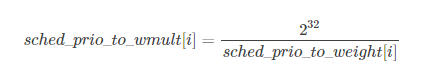
  进程每减少一个nice值，权重增加， 则多获得10%的CPU时间；每增加一个nice值，权重减少，则放弃10%的CPU时间。为执行该策略， 内核需要将优先级转换为权重值， 并提供了一张优先级->权重转换表sched_prio_to_weight，内核不仅维护了负荷权重自身，还保存另外一个数值，用于负荷重除的结果，即sched_prio_to_wmult数组，这两个数组中的数据是一一对应的。

const int sched_prio_to_weight[40] = {
/* -20 */     88761,     71755,     56483,     46273,     36291,
/* -15 */     29154,     23254,     18705,     14949,     11916,
/* -10 */      9548,      7620,      6100,      4904,      3906,
/*  -5 */      3121,      2501,      1991,      1586,      1277,
/*   0 */      1024,       820,       655,       526,       423,
/*   5 */       335,       272,       215,       172,       137,
/*  10 */       110,        87,        70,        56,        45,
/*  15 */        36,        29,        23,        18,        15,
};

const u32 sched_prio_to_wmult[40] = {
/* -20 */     48388,     59856,     76040,     92818,    118348,
/* -15 */    147320,    184698,    229616,    287308,    360437,
/* -10 */    449829,    563644,    704093,    875809,   1099582,
/*  -5 */   1376151,   1717300,   2157191,   2708050,   3363326,
/*   0 */   4194304,   5237765,   6557202,   8165337,  10153587,
/*   5 */  12820798,  15790321,  19976592,  24970740,  31350126,
/*  10 */  39045157,  49367440,  61356676,  76695844,  95443717,
/*  15 */ 119304647, 148102320, 186737708, 238609294, 286331153,
};

权重和nice公式：

例如：
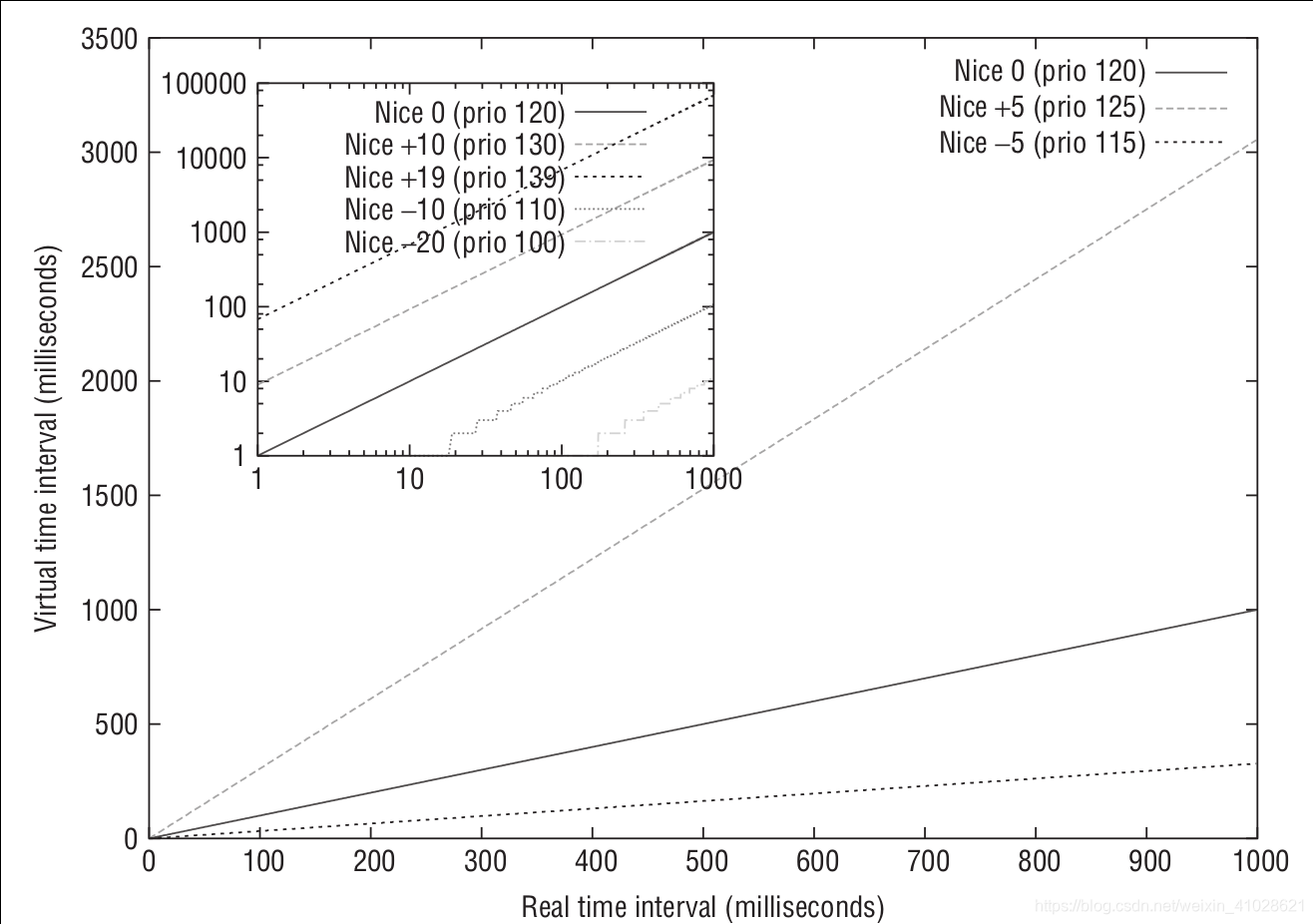
  两个进程A和B在nice级别0，即静态优先级120运行，因此两个进程的CPU份额相同，都是50%，nice级别为0的进程， 查其权重表可知是1024。每个进程的份额是1024/(1024+1024)=0.5， 即50%。

  如果进程B的优先级+1(优先级降低), 成为nice=1, 那么其CPU份额应该减少10%, 换句话说进程A得到的总的CPU应该是55%, 而进程B应该是45%. 优先级增加1导致权重减少, 即1024/1.25=820, 而进程A仍旧是1024, 则进程A现在将得到的CPU份额是1024/(1024+820=0.55, 而进程B的CPU份额则是820/(1024+820)=0.45. 这样就正好产生了10%的差值。

sched_prio_to_wmult和sched_prio_to_weight公式：

3. CFS基本原理

  基本原理：如果当前有n个进程需要调度执行，那么调度器应该在一个比较小的时间范围内，把这n个进程全都调度执行一遍，并且它们平分cpu时间，这样就可以做到所有进程的公平调度。那么这个比较小的时间就是任意一个R状态进程被调度的最大延时时间，即：任意一个R状态进程，都一定会在这个时间范围内被调度。这个时间叫做调度周期（sched_latency_ns）。进程越多，每个进程在周期内被执行的时间就会被平分的越小。调度器只需要对所有进程维护一个累积占用CPU时间数，就可以衡量出每个进程目前占用的CPU时间总量是不是过大或者过小，这个数字记录在每个进程的vruntime中。所有待执行进程都以vruntime为key放到一个由红黑树组成的队列中，每次被调度执行的进程，都是这个红黑树的最左子树上的那个进程，即vruntime时间最少的进程，这样就保证了所有进程的相对公平。

3.1.调度器配置参数

1.调度延迟时间
  CFS调度器的调度延迟时间不是固定的。当系统处于就绪态的进程少于一个定值（默认值8）的时候，调度延迟也是固定一个值不变（默认值6ms）。当系统就绪态进程个数超过这个值时，我们保证每个进程至少运行一定的时间才让出cpu。这个“至少一定的时间”被称为最小粒度时间。在CFS默认设置中，最小粒度时间是0.75ms。用变量sysctl_sched_min_granularity记录。因此，调度周期是一个动态变化的值。调度周期计算函数是__sched_period()。

• sched_latency_ns：This tuneable decides the scheduler period, the period in which all run queue tasks are scheduled at least once.
• sched_min_granularity_ns ：This tuneable decides the minimum time a task will be be allowed to run on CPU before being pre-empted out.

scheduler period有两种情况：

• number of runnable tasks < sched_nr_latency
  scheduler period = sched_latency_ns
• number of runnable tasks > sched_nr_latency
  scheduler period = number_of_running_tasks * sched_min_granularity_ns

    54 unsigned int sysctl_sched_latency           = 6000000ULL;                                              
    55 unsigned int normalized_sysctl_sched_latency        = 6000000ULL;
    
    75 unsigned int sysctl_sched_min_granularity       = 750000ULL;                                           
    76 unsigned int normalized_sysctl_sched_min_granularity    = 750000ULL;
    81 static unsigned int sched_nr_latency = 8;

   662 static u64 __sched_period(unsigned long nr_running)
   663 {
   664     if (unlikely(nr_running > sched_nr_latency))
   665         return nr_running * sysctl_sched_min_granularity;
   666     else
   667         return sysctl_sched_latency;
   668 }

3.2.Vruntime
  Virtual run time is the weighted time a task has run on the CPU.vruntime is measured in nano seconds.

一个进程的实际运行时间和虚拟运行时间之间的关系为:

vriture_runtime = wall_time(实际运行时间 ) * (NICE_0_LOAD / weight).
(NICE_0_LOAD = 1024, 表示nice值为0的进程权重)

如下所示，进程权重越大, 运行同样的实际时间, vruntime增长的越慢。

一个进程在一个调度周期内的虚拟运行时间大小为:

vruntime = 进程在一个调度周期内的实际运行时间 * NICE_0_LOAD / 进程权重
= (调度周期 * 进程权重 / 所有进程总权重) * NICE_0_LOAD / 进程权重
= 调度周期 * NICE_0_LOAD / 所有可运行进程总权重

  如上所示，一个进程在一个调度周期内的vruntime值大小是不和该进程自己的权重相关的，所以所有进程的vruntime值大小都是一样的。

3.3.就绪队列（runqueue）

  系统中每个CPU都会有一个全局的就绪队列（cpu runqueue），使用struct rq结构体描述，它是per-cpu类型，即每个cpu上都会有一个struct rq结构体。每一个调度类也有属于自己管理的就绪队列。例如，struct cfs_rq是CFS调度类的就绪队列，管理就绪态的struct sched_entity调度实体，后续通过pick_next_task接口从就绪队列中选择最适合运行的调度实体（虚拟时间最小的调度实体）。struct rt_rq是实时调度器就绪队列。struct dl_rq是Deadline调度器就绪队列。

参考资料：
https://notes.shichao.io/lkd/ch4/
http://www.wowotech.net/process_management/process-priority.html