Python数据分析：scikit-image

Python数据分析：scikit-image

scikit-image

• Python中用来进行图像处理的常用包之一
• 图像数据通过numpy中的ndarray表示
• 通常和numpy、SciPy共同使用进行图像数据的处理

skimage的图像数据

• skimage中的图像数据是由numpy的多维数组表示
• 由skimage加载的图像数据可以调用其他常用的包进行处理和计算，如matplotlib、SciPy等

数据类型和像素值

• CV中图像的像素值通常有以下两种处理范围

  1. 0 - 255,0：黑色， 255：白色
  2. 0 -1 ， 0：黑色， 1：白色

• skimage支持以上两种像素范围，根据数组的dtype选择使用

  1. float – 0 - 1
  2. unsigned bytes-- 0 - 255
  3. unsigned 16-bit integers – 0 - 65535

• 像素值数据类型转换

  • img_as_float, img_as_ubyte

• 推荐使用float，skimage包内部大部分用的是float类型，即像素值是0 - 1

显示图像

• 通过matplotlib， plt.imshow() , 可以指定不同的color map

图像I/O

• 加载图像，skimage.io.imread()
• 同时加载多个图像， skimage.io.imread_collection()
• 保存图像，skimage.io.imsave()

图像数据

• 图像数据是多维数组，前两维表示图像的高、宽，第三维表示图像的通道个数。灰度图像没有第三维度
• 分割和索引，可以像ndarray一样操作

色彩空间

• RGB,HSV,Gray…
• RGB转Gray，skimage.color.rgb2gray()

颜色直方图

• 直方图是一种能快速描述图像整体像素值分布的统计信息，skimage.exposure.histogram

对比度

• 增强图像数据的对比度有利于特征的提取，不论是从肉眼或是算法来看都有帮助

• 更改对比度范围

  skimage.exposure.rescale_intensity(image,in_range=(min, max))

  原图像数据中，小于min的像素值设为0，大于max的像素值设为255

• 直方图均衡化

  自动调整图像的对比度 skimage.exposure.equalize_hist(image) 均衡化后的图像数据范围是[0,1]

图像滤波

• 滤波是处理图像数据的常用基本操作
• 滤波操作可以去除图像中的噪声点，由此增强图像的特征

中值滤波 skimage.filters.rank.median

高斯滤波 skimage.filters.gaussian

import numpy as np
from matplotlib import pyplot as plt

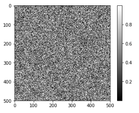
# 随机生成500x500的多维数组
random_image = np.random.random([500, 500])
plt.imshow(random_image, cmap='gray')
plt.colorbar()

运行：

from skimage import data

# 加载skimage中的coin数据
coins = data.coins()

print(type(coins), coins.dtype, coins.shape)
plt.imshow(coins, cmap='gray')
plt.colorbar()

运行：

cat = data.chelsea()
print("图片形状:", cat.shape)
print("最小值/最大值:", cat.min(), cat.max())

plt.imshow(cat)
plt.colorbar()

运行：

# 在图片上叠加一个红色方块
cat[10:110, 10:110, :] = [255, 0, 0]  # [red, green, blue]
plt.imshow(cat)

运行：

# 生成0-1间的2500个数据
linear0 = np.linspace(0, 1, 2500).reshape((50, 50))

# 生成0-255间的2500个数据
linear1 = np.linspace(0, 255, 2500).reshape((50, 50)).astype(np.uint8)

print("Linear0:", linear0.dtype, linear0.min(), linear0.max())
print("Linear1:", linear1.dtype, linear1.min(), linear1.max())

fig, (ax0, ax1) = plt.subplots(1, 2)
ax0.imshow(linear0, cmap='gray')
ax1.imshow(linear1, cmap='gray')

运行：

from skimage import img_as_float, img_as_ubyte

image = data.chelsea()

image_float = img_as_float(image) # 像素值范围：0-1
image_ubyte = img_as_ubyte(image) # 像素值范围：0-255

print("type, min, max:", image_float.dtype, image_float.min(), image_float.max())
print("type, min, max:", image_ubyte.dtype, image_ubyte.min(), image_ubyte.max())

print("231/255 =", 231/255.) # 验证0-255 转换到 0-1

运行：

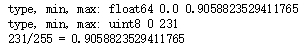
import matplotlib.pyplot as plt
import numpy as np
from skimage import data

image = data.camera()

fig, (ax_jet, ax_gray) = plt.subplots(ncols=2, figsize=(10, 5))

# 使用不同的color map
ax_jet.imshow(image, cmap='jet')
ax_gray.imshow(image, cmap='gray');

运行：

# 通过数组切片操作获取人脸区域
face = image[80:160, 200:280]
fig, (ax_jet, ax_gray) = plt.subplots(ncols=2)
ax_jet.imshow(face, cmap='jet')
ax_gray.imshow(face, cmap='gray');

运行：

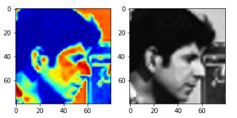
from skimage import io
image = io.imread('./images/balloon.jpg')

print(type(image))
plt.imshow(image);

运行：

# 同时加载多个图像
ic = io.imread_collection('./images/*.jpg')

f, axes = plt.subplots(nrows=1, ncols=len(ic), figsize=(15, 10))

for i, image in enumerate(ic):
    axes[i].imshow(image)
    axes[i].axis('off')
    
# 保存图像
saved_img = ic[0]
io.imsave('./output/ballet.jpg', saved_img)

运行：

import numpy as np
import matplotlib.pyplot as plt
%matplotlib inline
from skimage import data

color_image = data.chelsea()

print(color_image.shape)
plt.imshow(color_image)

运行：

red_channel = color_image[:, :, 0]  # 红色通道
plt.imshow(red_channel, cmap='gray')
print(red_channel.shape)

运行：

import skimage
#RGB--Gray
gray_img = skimage.color.rgb2gray(color_image)
plt.imshow(gray_img, cmap='gray')
print(gray_img.shape)

运行：

from skimage import data
from skimage import exposure

# 灰度图颜色直方图
image = data.camera()

hist, bin_centers = exposure.histogram(image)
fig, ax = plt.subplots(ncols=1)
ax.fill_between(bin_centers, hist)

运行：

# 彩色图像直方图
cat = data.chelsea()

# R通道
hist_r, bin_centers_r = exposure.histogram(cat[:,:,0])
# G通道
hist_g, bin_centers_g = exposure.histogram(cat[:,:,1])
# B通道
hist_b, bin_centers_b = exposure.histogram(cat[:,:,2])

fig, (ax_r, ax_g, ax_b) = plt.subplots(ncols=3, figsize=(10, 5))
ax_r.fill_between(bin_centers_r, hist_r)
ax_g.fill_between(bin_centers_g, hist_g)
ax_b.fill_between(bin_centers_b, hist_b)

运行：

# 原图像
image = data.camera()
hist, bin_centers = exposure.histogram(image)

# 改变对比度
# image中小于10的像素值设为0，大于180的像素值设为255
high_contrast = exposure.rescale_intensity(image, in_range=(10, 180))
hist2, bin_centers2 = exposure.histogram(high_contrast)

# 图像对比 
fig, (ax_1, ax_2) = plt.subplots(ncols=2, figsize=(10, 5))
ax_1.imshow(image, cmap='gray')
ax_2.imshow(high_contrast, cmap='gray')

fig, (ax_hist1, ax_hist2) = plt.subplots(ncols=2, figsize=(10, 5))
ax_hist1.fill_between(bin_centers, hist)
ax_hist2.fill_between(bin_centers2, hist2)

运行：

# 直方图均衡化
equalized = exposure.equalize_hist(image)
hist3, bin_centers3 = exposure.histogram(equalized)

# 图像对比 
fig, (ax_1, ax_2) = plt.subplots(ncols=2, figsize=(10, 5))
ax_1.imshow(image, cmap='gray')
ax_2.imshow(equalized, cmap='gray')

fig, (ax_hist1, ax_hist2) = plt.subplots(ncols=2, figsize=(10, 5))
ax_hist1.fill_between(bin_centers, hist)
ax_hist2.fill_between(bin_centers3, hist3)

运行：

from skimage import data
from skimage.morphology import disk
from skimage.filters.rank import median

img = data.camera()
med1 = median(img, disk(3)) # 3x3中值滤波
med2 = median(img, disk(5)) # 5x5中值滤波

# 图像对比 
fig, (ax_1, ax_2, ax_3) = plt.subplots(ncols=3, figsize=(15, 10))
ax_1.imshow(img, cmap='gray')
ax_2.imshow(med1, cmap='gray')
ax_3.imshow(med2, cmap='gray')

运行：

from skimage import data
from skimage.morphology import disk
from skimage.filters import gaussian

#高斯滤波
img = data.camera()
gas1 = gaussian(img, sigma=3) # sigma=3
gas2 = gaussian(img, sigma=5) # sigma=5

# 图像对比 
fig, (ax_1, ax_2, ax_3) = plt.subplots(ncols=3, figsize=(15, 10))
ax_1.imshow(img, cmap='gray')
ax_2.imshow(gas1, cmap='gray')
ax_3.imshow(gas2, cmap='gray')

运行：