matlab矩阵奇异值分解法,矩阵的奇异值分解 - 奋斗吧，骚年 - OSCHINA - 中文开源技术交流社区...

定义

矩阵的奇异值分解，顾名思义，是矩阵分解的一种。定义如下：

In linear algebra, the singular value decomposition (SVD) is a factorization of a real or complex matrix. It has many useful applications in signal processing and statistics.

Formally, the singular value decomposition of an m × n real or complex matrix M is a factorization of the form M = UΣV∗, where U is an m × m real or complex unitary matrix, Σ is an m × n rectangular diagonal matrix with non-negative real numbers on the diagonal, and V∗ (the conjugate transpose of V, or simply the transpose of V if V is real) is an n × n real or complex unitary matrix. The diagonal entries Σi,i of Σ are known as the singular values of M. The m columns of U and the n columns of V are called the left-singular vectors and right-singular vectors of M, respectively.

那么奇异值分解和特征值分解是什么关系呢？

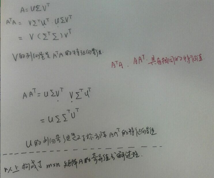
The singular value decomposition and the eigendecomposition are closely related. Namely:

The left-singular vectors of M are eigenvectors of MM∗.

The right-singular vectors of M are eigenvectors of M∗M.

The non-zero singular values of M (found on the diagonal entries of Σ) are the square roots of the non-zero eigenvalues of both M∗M and MM∗.

思路总结如下：

尤其需要注意外积形式的SVD

A=u1*c1*v1'+u2*c2*v2'+……+uk*ck*vk'

应用前景

在机器学习领域，有相当多的应用与奇异值都可以扯上关系，比如做feature reduction的PCA，做数据压缩(以图像压缩为代表)的算法，还有做搜索引擎语义层次检索的LSI(Latent Semantic Indexing)

调用代码

在matlab中可以直接调用svd()函数即可。

>> A=[1 2;3 4; 5 6;7 8]

A =

1     2

3     4

5     6

7     8

>> size(A)

ans =

4     2

>> svd(A)

ans =

14.2691

0.6268

>> [U,S,V]=svd(A)

U =

-0.1525   -0.8226   -0.3945   -0.3800

-0.3499   -0.4214    0.2428    0.8007

-0.5474   -0.0201    0.6979   -0.4614

-0.7448    0.3812   -0.5462    0.0407

S =

14.2691         0

0    0.6268

0         0

0         0

V =

-0.6414    0.7672

-0.7672   -0.6414

图像处理

svd可以运用到许多的领域，如搜索引擎算法，图像处理，人脸识别，等等。下面以图像处理为例，进行说明。

>> A=imread('56039.JPG');

>> I = mat2gray(A);

>> M=I(:,:,1);

>> [U,S,V]=svd(M);

>> M_100=U(:,1:100)*S(1:100,1:100)*V(:,1:100)';

>> imshow(M_100)

>> M_200=U(:,1:200)*S(1:200,1:200)*V(:,1:200)';

>> imshow(M_200)

>> M_300=U(:,1:300)*S(1:300,1:300)*V(:,1:300)';

>> imshow(M_300)

>> M_10=U(:,1:10)*S(1:10,1:10)*V(:,1:10)';

>> imshow(M_10)

>> ttr1svd(I);

>> imshow(U)

>> imshow(S)

>> imshow(V)

Warning: Image is too big to fit on screen; displaying at 67%

> In imuitools\private\initSize at 72

In imshow at 283

>> BB=U*S*V';

>> imshow(BB)

We can represent images as matrices. Consider an image having n times m pixels. For gray scale images, we need one number per pixel, which can be represented as a n times m matrix. For color images, we need three numbers per pixel, for each color: red, green and blue (RGB). Each color can be represented as a n times m matrix, and we can represent the full color image as a n times 3m matrix, where we stack each color’s matrix column-wise alongside of each other, as A=[A_{rm red},A_{rm green},A_{rm blue}].Using the low-rank approximation via SVD method, we can form the best rank-k approximations for the matrix.