基于 Python 的地理空间绘图指南（以 gma 空间绘图功能为例）

本文链接：https://blog.csdn.net/weixin_42155937/article/details/130022671

1 gma 简介

gma 是一个基于 Python 的地理、气象数据快速处理和数据分析函数包（Geographic and Meteorological Analysis，gma）。gma 网站：地理与气象分析库。

gma 的主要功能有哪些？

气候气象（例如 SPEI、SPI、ET0 等）。
遥感指数（例如 NDVI、EVI、TVDI 等）。
数学运算（例如数据平滑、评估、滤波、拉伸、增强变换等）。
系统交互（例如获取路径、重命名、压缩等操作）。
空间杂项（例如计算空间距离、面积计算，坐标转换、空间插值等操作）。
栅格处理（例如栅格镶嵌、裁剪、重采样、重投影、格式转换、数据融合等）。
栅格分析（例如 DEM 坡度、坡向、阴影、等值线等计算）。
矢量处理（例如矢量裁剪、擦除、交集、融合、重投影等）。
地图工具（例如栅格、矢量数据绘图，指北针、比例尺等生成，坐标系定义等）

本文所用的 gma 版本及下载

目前，本文所用的 gma 版本为 gma-1.1.5a15。

系统 (X64)： Window 10+
Python 版本： 3.10.9

下载地址：

链接：https://pan.baidu.com/s/12wyfOGo0IMsIQIca7iOrxg?pwd=9scj
提取码：9scj

其他版本可使用 pip install gma 安装

2 发展历程

gma 绘图功能以 ArcGIS 绘图功能为参考，目标是构建一个以 Python 为基础的快速地理绘图工具。
其大约与2022 年 11 月疫情居家期间开始构建，目前开放（指的是可以直接调用，且有使用帮助的）功能包括：

plot：主要功能是创建地图框。
rcs: 为配合绘图功能，构建的扩展空间参考模块。目的在于初始化已有坐标系，并创建自定义坐标系。
inres：内置资源模块，主要提供 gma 内置的一些矢量数据、栅格数据，方便底图添加。

从 1.1.2 版本开始，gma 绘图功能的主要更新说明如下：

1.1.2：新增 map 地图工具包，开始支持空间绘图（基于 gma 的矢量图层（Layer）和栅格数据集类（DataSet））。
1.1.3：添加栅格数据集绘制功能（离散型栅格）等。
1.1.4：添加栅格数据集绘制功能（重分类或唯一值栅格）等，开始内置一些底图数据（世界国家、世界陆地和海洋DEM）。
1.1.5（将在2023年4月的某个周末发布）：添加矢量要素（Feature）绘制功能，添加更多的地图数据（湖泊、陆地、河流、海洋以及自然地球影像）。

其中也伴随着众多 BUG 修复和功能优化，以及一些配套函数的构建，例如（以下函数均位于gma.io 模块下）：

CreateFeatureFromPoints：根据坐标点创建 Feature（然后可按照矢量要素的方法添加）
CreateLayerFromFeature：将多个Feature 合并生成 Layer（然后可按照矢量图层方法添加）
ReadArrayAsDataSet：将数组读取为 DataSet（然后可按照栅格数据集的方式添加）
TranslateFeatureToDataSet：将矢量要素转换为栅格数据集（类似于矢量转栅格）
TranslateLayerToDataSet：将矢量图层转换为栅格数据集（类似于矢量转栅格）

3 主要绘图思路与步骤

第一步：添加一个地图框。与 ArcGIS 地图框类似，后续所有数据均在地图框内添加和绘制。
第二步：添加数据（包括矢量图层、矢量要素、栅格数据集等）、并配置参数（颜色、大小、宽度等）。与ArcGIS 类似，这些数据在添加到地图框后均会被重投影到地图框配置的底图坐标系上；可配置的参数类似ArcGIS的符号系统，例如矢量数据的背景色、边界色等，栅格数据的色带（颜色条）、拉伸方式（例如直方图均衡化）和数据变换（例如 gamma 变换）等。
第三步：添加地图整饰要素（例如：指北针、比例尺和图例等）。与 ArcGIS 的地图整饰要素类似，可通过参数控制颜色、大小、样式等。

4 主要绘图功能示例（gma 1.1.5 +）

from gma.map import rcs, plot, inres

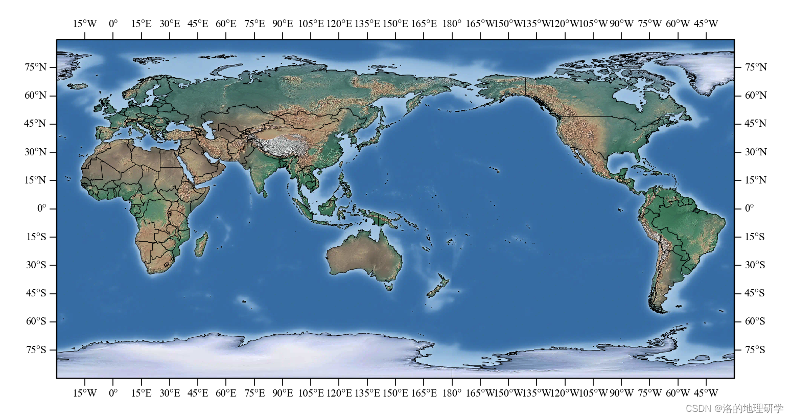
4.1 绘制包含国界线的自然地球图

# 1.初始化一个地图框，底图为 WGS84 坐标系
MapF = plot.MapFrame(Axes = None, BaseMapProj = 'WGS84', Extent = None)

# 2.将内置的世界矢量图层添加到地图框
# 2.1 添加内置国界（矢量数据），并设置填充色透明，线宽 0.2，线黑色
MapL1 = MapF.AddLayer(inres.WorldLayer.Country, FaceColor = 'none', LineWidth = 0.2, EdgeColor = 'black', Zorder = 1)
# 2.2 添加自然地球底图（RGB 栅格，不需要配置色带）
MapD1 = MapF.AddDataSetDiscrete(inres.WorldDataSet.NaturalEarth)

# 3.获取经纬网，但不显示经纬网，为地图框刻度使用
GridLines = MapF.AddGridLines(LineColor = 'none')

# 4. 设置地图框边框
Frame = MapF.SetFrame()

4.2 绘制陆地、海洋、河流和湖泊数据

# 1.初始化一个地图框，底图为 WGS84 坐标系
MapF = plot.MapFrame(Axes = None, BaseMapProj = 'WGS84', Extent = None)

# 2.将内置的世界矢量图层添加到地图框
MapL1 = MapF.AddLayer(inres.WorldLayer.Land, FaceColor = 'white', LineWidth = 0.2, EdgeColor = 'black')
MapL2 = MapF.AddLayer(inres.WorldLayer.Lake, FaceColor = 'lightblue', LineWidth = 0.2, EdgeColor = '#BEE8FF', Zorder = 2)
MapL3 = MapF.AddLayer(inres.WorldLayer.River, LineColor = 'lightblue', LineWidth = 0.2, Zorder = 3)
MapL4 = MapF.AddLayer(inres.WorldLayer.Ocean, FaceColor = '#BEE8FF', EdgeColor = 'none')

# 3.获取经纬网，但不显示经纬网，为地图框刻度使用
GridLines = MapF.AddGridLines(LineColor = 'none')

# 4. 设置地图框边框
Frame = MapF.SetFrame()

4.3 最好把中国放在地图中央

# 0 使用 gma 定义一个中心经线为 150°E 的简易圆柱投影（即：改变了中央经线的地理坐标系）
Proj = rcs.CustomGCS(CentralLongitude = 150)

# 1.初始化一个地图框，底图 0 定义的坐标系
MapF = plot.MapFrame(Axes = None, BaseMapProj = Proj, Extent = None)

# 2.将内置的世界矢量图层添加到地图框
MapL1 = MapF.AddLayer(inres.WorldLayer.Land, FaceColor = 'white', LineWidth = 0.2, EdgeColor = 'black')
MapL2 = MapF.AddLayer(inres.WorldLayer.Lake, FaceColor = 'lightblue', LineWidth = 0.2, EdgeColor = '#BEE8FF', Zorder = 2)
MapL3 = MapF.AddLayer(inres.WorldLayer.River, LineColor = 'lightblue', LineWidth = 0.2, Zorder = 3)
MapL4 = MapF.AddLayer(inres.WorldLayer.Ocean, FaceColor = '#BEE8FF', EdgeColor = 'none')

# 3.获取经纬网，但不显示经纬网，为地图框刻度使用
GridLines = MapF.AddGridLines(LineColor = 'none')

# 4. 设置地图框边框
Frame = MapF.SetFrame()

4.4 为添加的栅格数据集进行拉伸和变换（数据增强）

4.4.1 拉伸数据集（以百分比截断拉伸为例）

# 0 使用 gma 定义一个中心经线为 150°E 的简易圆柱投影（即：改变了中央经线的地理坐标系）
Proj = rcs.CustomGCS(CentralLongitude = 150)

# 1.初始化一个地图框，底图 0 定义的坐标系
MapF = plot.MapFrame(Axes = None, BaseMapProj = Proj, Extent = None)

# 2.将内置的世界矢量图层添加到地图框
# 2.1 添加内置国界（矢量数据），并设置填充色透明，线宽 0.2，线黑色
MapL1 = MapF.AddLayer(inres.WorldLayer.Country, FaceColor = 'none', LineWidth = 0.2, EdgeColor = 'black', Zorder = 1)
# 2.2 添加自然地球底图，并对数据进行百分比截断拉伸（相关参数详见：gma.math.Stretch）
MapD1 = MapF.AddDataSetDiscrete(inres.WorldDataSet.NaturalEarth, Stretch = 'Percentage')

# 3.获取经纬网，但不显示经纬网，为地图框刻度使用
GridLines = MapF.AddGridLines(LineColor = 'none')

# 4. 添加地图框边框
Frame = MapF.SetFrame()

4.4.2 变换数据集（以 Gamma 变换为例）

# 0 使用 gma 定义一个中心经线为 150°E 的简易圆柱投影（即：改变了中央经线的地理坐标系）
Proj = rcs.CustomGCS(CentralLongitude = 150)

# 1.初始化一个地图框，底图 0 定义的坐标系
MapF = plot.MapFrame(Axes = None, BaseMapProj = Proj, Extent = None)

# 2.将内置的世界矢量图层添加到地图框
# 2.1 添加内置国界（矢量数据），并设置填充色透明，线宽 0.2，线黑色
MapL1 = MapF.AddLayer(inres.WorldLayer.Country, FaceColor = 'none', LineWidth = 0.2, EdgeColor = 'black', Zorder = 1)
# 2.2 添加自然地球底图，并对数据进行 gamma 变换，并设置变换值（相关参数详见：gma.math.Correction）
MapD1 = MapF.AddDataSetDiscrete(inres.WorldDataSet.NaturalEarth, Correction = 'Gamma', CorrectionPROP = dict(GammaV = 2))

# 3.获取经纬网，但不显示经纬网，为地图框刻度使用
GridLines = MapF.AddGridLines(LineColor = 'none')

# 4. 添加地图框边框
Frame = MapF.SetFrame()

4.5 绘制单波段数据集，并为其配置色带

# 0 使用 gma 定义一个中心经线为 150°E 的简易圆柱投影（即：改变了中央经线的地理坐标系）
Proj = rcs.CustomGCS(CentralLongitude = 150)

# 1.初始化一个地图框，底图 0 定义的坐标系
MapF = plot.MapFrame(Axes = None, BaseMapProj = Proj, Extent = None)

# 2.将内置的世界矢量图层添加到地图框
# 2.1 添加内置国界（矢量数据），并设置填充色透明，线宽 0.2，线黑色
MapL1 = MapF.AddLayer(inres.WorldLayer.Country, FaceColor = 'none', LineWidth = 0.2, EdgeColor = 'black', Zorder = 1)
# 2.2 添加世界陆地和海洋 DEM ，并配置 jet 色带
MapD1 = MapF.AddDataSetDiscrete(inres.WorldDataSet.DEM, CMap = 'jet')

# 3.获取经纬网，但不显示经纬网，为地图框刻度使用
GridLines = MapF.AddGridLines(LineColor = 'none')

# 4. 添加地图框边框
Frame = MapF.SetFrame()

4.6 在地图上绘制点、线、面

Points = [[112.5, 34.4], [30, 60], [2.3, 48.8], [47.5, -18.9]]
# 创建点、线、面 Feature
FPoints = plot.CreatePlotFeature(Points, Type = 'MultiPoint')
FLine = plot.CreatePlotFeature(Points, Type = 'Line')
FPolygon = plot.CreatePlotFeature(Points, Type = 'Polygon')

# 1.初始化一个地图框
MapF = plot.MapFrame(Axes = None, BaseMapProj = Proj, Extent = None)

# 2.将内置的世界矢量图层添加到地图框
MapD1 = MapF.AddDataSetDiscrete(inres.WorldDataSet.NaturalEarth, Zorder = 0)
# 2.2 添加面、线、点
MapL1 = MapF.AddFeature(FPolygon, FaceColor = (0.8, 0.5, 0.5, 0.5), Zorder = 1)
MapL2 = MapF.AddFeature(FLine, LineColor = 'green', LineWidth = 0.5, Zorder = 2)
MapL3 = MapF.AddFeature(FPoints, PointColor = 'red', PointSize = 2, Zorder = 3)

MapF.AddGridLines(LineColor = 'none')
Frame = MapF.SetFrame()

4.7 换个视角看一下

Points = [[112.5, 34.4], [30, 60], [2.3, 48.8], [47.5, -18.9]]
# 创建点、线、面 Feature
FPoints = plot.CreatePlotFeature(Points, Type = 'MultiPoint')
FLine = plot.CreatePlotFeature(Points, Type = 'Line')
FPolygon = plot.CreatePlotFeature(Points, Type = 'Polygon')

# 0 使用 gma 定义一个中心经线为 112°E 的 Albers 等面积投影
Proj = rcs.AlbersEqualArea(CentralLongitude = 112)

# 1.初始化一个地图框，底图 0 定义的坐标系
MapF = plot.MapFrame(Axes = None, BaseMapProj = Proj, Extent = None)

# 2.将内置的世界矢量图层添加到地图框
MapD1 = MapF.AddDataSetDiscrete(inres.WorldDataSet.NaturalEarth, Zorder = 0)
# 2.2 添加面、线、点
MapL1 = MapF.AddFeature(FPolygon, FaceColor = (0.8, 0.5, 0.5, 0.5), Zorder = 1)
MapL2 = MapF.AddFeature(FLine, LineColor = 'green', LineWidth = 0.5, Zorder = 2)
MapL3 = MapF.AddFeature(FPoints, PointColor = 'red', PointSize = 2, Zorder = 3)

MapF.AddGridLines(LineColor = 'none')
Frame = MapF.SetFrame()

5 从空间插值到地图绘制全过程

5.1 从反距离权重插值到绘图

示例数据下载：

链接：https://pan.baidu.com/s/1-lNWdo-V5bsa1r5JS_N4wg?pwd=agzp
提取码：agzp

5.1.1 读取数据并插值

# import gma
import pandas as pd
from gma import io
from gma.smc import Interpolate
from gma.map import rcs, plot, inres

Data = pd.read_excel("Interpolate.xlsx")
Points = Data.loc[:, ['经度','纬度']].values
Values = Data.loc[:, ['值']].values

# 步骤1：反距离权重插值
IDWD = Interpolate.IDW(Points, Values, Resolution = 0.01, InProjection = 'WGS84')

# 步骤2：将插值结果转换为 DataSet 数据集
IDWDataSet = io.ReadArrayAsDataSet(IDWD.Data, Projection = 'WGS84', Transform = IDWD.Transform)

5.1.2 绘图（离散型）

# 步骤3：绘图
# 0 使用 gma 定义一个中心经线为 125°E ，两条标准纬线为 40°N, 52°N 的 Albers 等面积投影
Proj = rcs.AlbersEqualArea(CentralLongitude = 125, StandardParallels = (40, 52))

# 1.初始化一个地图框，并配置视图范围 
MapF = plot.MapFrame(Axes = None, BaseMapProj = Proj, Extent = [112, 38, 138, 54])

# 2.将内置的世界矢量图层添加到地图框
MapL1 = MapF.AddLayer(inres.WorldLayer.Country, FaceColor = 'none', LineWidth = 0.2, EdgeColor = 'black', Zorder = 2)
MapL2 = MapF.AddLayer(inres.WorldLayer.Ocean, FaceColor = '#BEE8FF', EdgeColor = 'none')

MapD1 = MapF.AddDataSetDiscrete(IDWDataSet, CMap = 'jet', Zorder = 1)

# 3.获取经纬网
GridLines = MapF.AddGridLines(LONRange = (100, 150, 5), LATRange = (30, 60, 5))

# 4.设置地图框边框
Frame = MapF.SetFrame()

5.1.3 地图整饰要素（指北针、比例尺）修饰

# 0 使用 gma 定义一个中心经线为 125°E ，两条标准纬线为 40°N, 52°N 的 Albers 等面积投影
Proj = rcs.AlbersEqualArea(CentralLongitude = 125, StandardParallels = (40, 52))

# 1.初始化一个地图框，并配置视图范围 
MapF = plot.MapFrame(Axes = None, BaseMapProj = Proj, Extent = [112, 38, 138, 54])

# 2.将内置的世界矢量图层添加到地图框
MapL1 = MapF.AddLayer(inres.WorldLayer.Country, FaceColor = 'none', LineWidth = 0.2, EdgeColor = 'black', Zorder = 2)
MapL2 = MapF.AddLayer(inres.WorldLayer.Ocean, FaceColor = '#BEE8FF', EdgeColor = 'none')

MapD1 = MapF.AddDataSetDiscrete(IDWDataSet, CMap = 'jet', Zorder = 1)

# 3.获取经纬网
GridLines = MapF.AddGridLines(LONRange = (100, 150, 5), LATRange = (30, 60, 5))

# 4.添加地图整饰要素
AddCompass = MapF.AddCompass(LOC = (0.1, 0.8), Color = 'black')
ScaleBar = MapF.AddScaleBar(LOC = (0.1, 0.02), Width = 0.3, Color = 'black', FontSize = 7)

# 5.设置地图框边框
Frame = MapF.SetFrame()

5.1.4 绘制重分类图并添加图例

# 0 使用 gma 定义一个中心经线为 125°E ，两条标准纬线为 40°N, 52°N 的 Albers 等面积投影
Proj = rcs.AlbersEqualArea(CentralLongitude = 125, StandardParallels = (40, 52))

# 1.初始化一个地图框，并配置视图范围 
MapF = plot.MapFrame(Axes = None, BaseMapProj = Proj, Extent = [112, 38, 138, 54])

# 2.将内置的世界矢量图层添加到地图框
MapL1 = MapF.AddLayer(inres.WorldLayer.Country, FaceColor = 'none', LineWidth = 0.2, EdgeColor = 'black', Zorder = 2)
MapL2 = MapF.AddLayer(inres.WorldLayer.Ocean, FaceColor = '#BEE8FF', EdgeColor = 'none')

MapD1 = MapF.AddDataSetClassify(IDWDataSet,
                                CMap = 'jet',
                                Remap = [[-25, 0], [-20, 1], [-15, 2], [-10, 3],[-5, 4], [100, 5]],
                                Method = 'Range', 
                                Labels = ['<= -25', '-25 ~ -20', '-20 ~ -15','-15 ~ -10','-10 ~ -5',' > -5'],
                                Zorder = 1     
                               )

# 3.获取经纬网
GridLines = MapF.AddGridLines(LONRange = (100, 150, 5), LATRange = (30, 60, 5))

# 4.添加地图整饰要素
AddCompass = MapF.AddCompass(LOC = (0.1, 0.8), Color = 'black')
ScaleBar = MapF.AddScaleBar(LOC = (0.1, 0.02), Width = 0.3, Color = 'black', FontSize = 7)
Legend = MapF.AddLegend(LegendName = '气温（℃）', TitleAlignment = 'left', PlotID = [2], LOC = (0.75, 0.5), TitleFont = 'SimSun')

# 5.设置地图框边框
Frame = MapF.SetFrame()

5.2 其他插值方法（自然邻域法、克里金法、趋势面法、B-样条函数法）对比

import matplotlib.pyplot as plt

TD = Interpolate.Trend(Points, Values, Resolution = 0.1)
KD = Interpolate.Kriging(Points, Values, Resolution = 0.1)
NND = Interpolate.NaturalNeighbor(Points, Values, Resolution = 0.1)
BSD = Interpolate.BSpline(Points, Values, Resolution = 0.1)

TDDataSet = io.ReadArrayAsDataSet(TD.Data, Projection = 'WGS84', Transform = TD.Transform)
KDDataSet = io.ReadArrayAsDataSet(KD.Data, Projection = 'WGS84', Transform = KD.Transform)
NNDDataSet = io.ReadArrayAsDataSet(NND.Data, Projection = 'WGS84', Transform = NND.Transform)
BSDDataSet = io.ReadArrayAsDataSet(BSD.Data, Projection = 'WGS84', Transform = BSD.Transform)

# 0 使用 gma 定义一个中心经线为 125°E ，两条标准纬线为 40°N, 52°N 的 Albers 等面积投影
Proj = rcs.AlbersEqualArea(CentralLongitude = 125, StandardParallels = (40, 52))

PlotDS = [TDDataSet, KDDataSet, NNDDataSet, BSDDataSet]

Titles = ['Trend', 'Kriging', 'NaturalNeighbor', 'BSpline']

fig = plt.figure(figsize = (8, 6), dpi = 300)

for i in range(4):
    Axes = plt.subplot(2, 2, i + 1)

    # 1.初始化一个地图框，并配置视图范围 
    MapF = plot.MapFrame(Axes = Axes, BaseMapProj = Proj, Extent = [110, 38, 140, 54])

    # 2.将内置的世界矢量图层添加到地图框
    MapL1 = MapF.AddLayer(inres.WorldLayer.Country, FaceColor = 'none', LineWidth = 0.2, EdgeColor = 'black', Zorder = 2)
    MapL2 = MapF.AddLayer(inres.WorldLayer.Ocean, FaceColor = '#BEE8FF', EdgeColor = 'none')

    MapD1 = MapF.AddDataSetClassify(PlotDS[i],
                                    CMap = 'jet',
                                    Remap = [[-25, 0], [-20, 1], [-15, 2], [-10, 3],[-5, 4], [100, 5]],
                                    Method = 'Range', 
                                    Labels = ['<= -25', '-25 ~ -20', '-20 ~ -15','-15 ~ -10','-10 ~ -5',' > -5'],
                                    Zorder = 1     
                                   )

    # 3.获取经纬网
    GridLines = MapF.AddGridLines(LONRange = (100, 150, 5), LATRange = (30, 60, 5))

    # 4.添加地图整饰要素
    AddCompass = MapF.AddCompass(LOC = (0.1, 0.75), Color = 'black')
    ScaleBar = MapF.AddScaleBar(LOC = (0.1, 0.02), Width = 0.3, Color = 'black', FontSize = 7)
    if i == 3:
        Legend = MapF.AddLegend(LegendName = '气温（℃）', 
                                TitleAlignment = 'left', 
                                LabelFontSize = 5, 
                                PlotID = [2], 
                                LOC = (0.74, 0.35), 
                                HandleLength = 2.3,
                                HandleHeight = 1.5,
                                TitleFontSize = 7,
                                TitleFont = 'SimSun')

    Frame = MapF.SetFrame()
     
    Axes.set_title(Titles[i], fontsize = 8, y = 0.85, fontdict = {'family':'Times New Roman'})
    
fig.subplots_adjust(wspace = 0.02, hspace = 0.01)

6 其他相关拓展

6.1 查看当前系统所有色带

DefinedCMaps = plot.GetPreDefinedCMaps(PlotCMap = True)

（部分图）

6.2 查看当前系统所有字体

SystemFonts = plot.GetSystemFonts(ShowFonts = True)