


- 🍨 本文为🔗365天深度学习训练营中的学习记录博客
- 🍖 原作者:K同学啊
一、前期准备
1.设置GPU
import torch
import torch.nn as nn
import torchvision.transforms as transforms
import torchvision
from torchvision import transforms,datasets
import os,PIL,pathlib,warnings
warnings.filterwarnings("ignore")
#忽略警告信息
device = torch.device("cuda" if torch.cuda.is_available()else "cpu")
device
device(type='cuda')
2.导入数据
import os,PIL,random,pathlib

data_dir='F:/jupyter lab/DL-100-days/datasets/IDL_photos/J3-data/'
data_dir = pathlib.Path(data_dir)
data_paths = list(data_dir.glob('*'))
classeNames =[str(path).split("\\")[6] for path in data_paths]
classeNames
['0', '1']
train_transforms = transforms.Compose([
    transforms.Resize([224, 224]),  # 将输入图片resize成统一尺寸
    transforms.ToTensor(),          # 将PIL Image或numpy.ndarray转换为tensor,并归一化到[0,1]之间
    transforms.Normalize(           # 标准化处理-->转换为标准正太分布(高斯分布),使模型更容易收敛
        mean=[0.485, 0.456, 0.406],
        std =[0.229, 0.224, 0.225])  # 其中 mean=[0.485,0.456,0.406]与std=[0.229,0.224,0.225] 从数据集中随机抽样计算得到的。
])

test_transforms = transforms.Compose([
    transforms.Resize([224, 224]),  # 将输入图片resize成统一尺寸
    transforms.ToTensor(),          # 将PIL Image或numpy.ndarray转换为tensor,并归一化到[0,1]之间
    transforms.Normalize(           # 标准化处理-->转换为标准正太分布(高斯分布),使模型更容易收敛
        mean=[0.485, 0.456, 0.406],
        std =[0.229, 0.224, 0.225])  # 其中 mean=[0.485,0.456,0.406]与std=[0.229,0.224,0.225] 从数据集中随机抽样计算得到的。
])

total_data = datasets.ImageFolder(data_dir, train_transforms)
total_data
Dataset ImageFolder
Number of datapoints: 13403
Root location: F:\jupyter lab\DL-100-days\datasets\IDL_photos\J3-data
StandardTransform
Transform: Compose(
Resize(size=[224, 224], interpolation=bilinear, max_size=None, antialias=None)
ToTensor()
Normalize(mean=[0.485, 0.456, 0.406], std=[0.229, 0.224, 0.225])
)
total_data.class_to_idx{'0': 0, '1': 1}
3.划分数据集
train_size = int(0.8 * len(total_data))
test_size  = len(total_data) - train_size
train_dataset, test_dataset = torch.utils.data.random_split(total_data, [train_size, test_size])
train_dataset,test_dataset
(<torch.utils.data.dataset.Subset at 0x1434649b340>, <torch.utils.data.dataset.Subset at 0x143d65aff10>)
batch_size = 32
train_dl = torch.utils.data.DataLoader(train_dataset,
                                            batch_size=batch_size,
                                            shuffle=True)
test_dl=torch.utils.data.DataLoader(test_dataset,
                                            batch_size=batch_size,
                                            shuffle=True)
for X,y in test_dl:
print("shape of X [N,C,H,W]:", X.shape)
print("shape of y:",y.shape, y.dtype)
breakshape of X [N,C,H,W]: torch.Size([32, 3, 224, 224]) shape of y: torch.Size([32]) torch.int64
三、构建网络模型
from collections import OrderedDict
import torch
import torch.nn as nn
import torch.nn.functional as F
1.DenseLayer模块
class DenseLayer(nn.Sequential):
    def __init__(self,in_channel,growth_rate,bn_size, drop_rate):
        super(DenseLayer,self).__init__()
        self.add_module('norm1',nn.BatchNorm2d(in_channel))
        self.add_module('relu1',nn.ReLU(inplace=True))
        self.add_module('conv1',nn.Conv2d(in_channel, bn_size*growth_rate,
                                          kernel_size=1, stride=1, bias=False))
        self.add_module('norm2',nn.BatchNorm2d(bn_size*growth_rate))
        self.add_module('relu2',nn.ReLU(inplace=True))
        self.add_module('conv2',nn.Conv2d(bn_size*growth_rate, growth_rate,
                                          kernel_size=3,stride=1,padding=1,bias=False))
        self.drop_rate = drop_rate

    def forward(self, x):
        new_feature=super(DenseLayer,self).forward(x)
        if self.drop_rate>0:
            new_feature = F.dropout(new_feature, p=self.drop_rate, training=self.training)
        return torch.cat([x,new_feature],1)
2.DenseBlock模块
''' DenseBlock '''
class DenseBlock(nn.Sequential):
    def __init__(self,num_layers,in_channel,bn_size, growth_rate, drop_rate):
        super(DenseBlock, self).__init__()
        for i in range(num_layers):
            layer = DenseLayer(in_channel+i*growth_rate, growth_rate, bn_size, drop_rate)
            self.add_module('denselayer%d'%(i+1,),layer)
3.Transition模块
''' Transition layer between two adjacent DenseBlock '''
class Transition(nn.Sequential):
    def __init__(self,in_channel,out_channel):
        super(Transition,self).__init__()
        self.add_module('norm',nn.BatchNorm2d(in_channel))
        self.add_module('relu',nn.ReLU(inplace=True))
        self.add_module('conv',nn.Conv2d(in_channel, out_channel, kernel_size=1, stride=1, bias=False))
        self.add_module('pool',nn.AvgPool2d(2,stride=2))
4.构建DenseNet
class DenseNet(nn.Module):
    def __init__(self,growth_rate=32,block_config=(6,12,24,16),init_channel=64,
                 bn_size=4,compression_rate=0.5,drop_rate=0,num_classes=1000):
        '''
        :param growth rate:(int)number of filters used in DenseLayer, `k` in the paper
        :param block config:(list of 4 ints)number of layers in eatch DenseBlock
        :param init channel:(int)number of filters in the first Conv2d
        :param bn_size:(int)the factor using in the bottleneck layer
        :param compression rate:(float)the compression rate used in Transition Layer
        :param drop rate:(float)the drop rate after each DenseLayer
        :param num_classes:(int) 待分类的类别数
        '''
        super(DenseNet,self).__init__()
        # first Conv2d
        self.features =nn.Sequential(OrderedDict([
            ('conv0',nn.Conv2d(3,init_channel,kernel_size=7,stride=2,padding=3, bias=False)),
            ('norm0',nn.BatchNorm2d(init_channel)),
            ('relu0',nn.ReLU(inplace=True)),
            ('pool0',nn.MaxPool2d(3, stride=2, padding=1))
        ]))

        # DenseBlock
        num_features = init_channel
        for i,num_layers in enumerate(block_config):
            block = DenseBlock(num_layers,num_features, bn_size, growth_rate, drop_rate)
            self.features.add_module('denseblock%d'%(i+1),block)
            num_features += num_layers*growth_rate
            if i != len(block_config)-1:
                transition = Transition(num_features,int(num_features*compression_rate))
                self.features.add_module('transition%d'%(i+1),transition)
                num_features =int(num_features*compression_rate)

        # final BN+ReLU
        self.features.add_module('norm5', nn.BatchNorm2d(num_features))
        self.features.add_module('relu5',nn.ReLU(inplace=True))
        #分类层
        self.classifier =nn.Linear(num_features,num_classes)

        #参数初始化
        for m in self.modules():
            if isinstance(m,nn.Conv2d):
                nn.init.kaiming_normal_(m.weight)
            elif isinstance(m, nn.BatchNorm2d):
                nn.init.constant(m.bias,0)
                nn.init.constant(m.weight, 1)
            elif isinstance(m,nn.Linear):
                nn.init.constant(m.bias,0)

    def forward(self,x):
        x= self.features(x)
        x=F.avg_pool2d(x,7,stride=1).view(x.size(0),-1)
        x=self.classifier(x)
        return x
5.构建densenet121
device ="cuda" if torch.cuda.is_available()else "cpu"
print("Using {} device".format(device))

densenet121 =DenseNet(init_channel=64,
                      growth_rate=32,
                      block_config=(6,12,24,16),
                      num_classes=len(classeNames))

model = densenet121.to(device)
model
Using cuda device
DenseNet(
(features): Sequential(
(conv0): Conv2d(3, 64, kernel_size=(7, 7), stride=(2, 2), padding=(3, 3), bias=False)
(norm0): BatchNorm2d(64, eps=1e-05, momentum=0.1, affine=True, track_running_stats=True)
(relu0): ReLU(inplace=True)
(pool0): MaxPool2d(kernel_size=3, stride=2, padding=1, dilation=1, ceil_mode=False)
(denseblock1): DenseBlock(
(denselayer1): DenseLayer(
(norm1): BatchNorm2d(64, eps=1e-05, momentum=0.1, affine=True, track_running_stats=True)
(relu1): ReLU(inplace=True)
(conv1): Conv2d(64, 128, kernel_size=(1, 1), stride=(1, 1), bias=False)
(norm2): BatchNorm2d(128, eps=1e-05, momentum=0.1, affine=True, track_running_stats=True)
(relu2): ReLU(inplace=True)
(conv2): Conv2d(128, 32, kernel_size=(3, 3), stride=(1, 1), padding=(1, 1), bias=False)
)
..........
(denselayer15): DenseLayer(
(norm1): BatchNorm2d(960, eps=1e-05, momentum=0.1, affine=True, track_running_stats=True)
(relu1): ReLU(inplace=True)
(conv1): Conv2d(960, 128, kernel_size=(1, 1), stride=(1, 1), bias=False)
(norm2): BatchNorm2d(128, eps=1e-05, momentum=0.1, affine=True, track_running_stats=True)
(relu2): ReLU(inplace=True)
(conv2): Conv2d(128, 32, kernel_size=(3, 3), stride=(1, 1), padding=(1, 1), bias=False)
)
(denselayer16): DenseLayer(
(norm1): BatchNorm2d(992, eps=1e-05, momentum=0.1, affine=True, track_running_stats=True)
(relu1): ReLU(inplace=True)
(conv1): Conv2d(992, 128, kernel_size=(1, 1), stride=(1, 1), bias=False)
(norm2): BatchNorm2d(128, eps=1e-05, momentum=0.1, affine=True, track_running_stats=True)
(relu2): ReLU(inplace=True)
(conv2): Conv2d(128, 32, kernel_size=(3, 3), stride=(1, 1), padding=(1, 1), bias=False)
)
)
(norm5): BatchNorm2d(1024, eps=1e-05, momentum=0.1, affine=True, track_running_stats=True)
(relu5): ReLU(inplace=True)
)
(classifier): Linear(in_features=1024, out_features=2, bias=True)
)
#统计模型参数量以及其他指标
import torchsummary as summary
summary.summary(model,(3,224,224))
----------------------------------------------------------------
Layer (type) Output Shape Param #
================================================================
Conv2d-1 [-1, 64, 112, 112] 9,408
BatchNorm2d-2 [-1, 64, 112, 112] 128
ReLU-3 [-1, 64, 112, 112] 0
MaxPool2d-4 [-1, 64, 56, 56] 0
BatchNorm2d-5 [-1, 64, 56, 56] 128
ReLU-6 [-1, 64, 56, 56] 0
Conv2d-7 [-1, 128, 56, 56] 8,192
BatchNorm2d-8 [-1, 128, 56, 56] 256
ReLU-9 [-1, 128, 56, 56] 0
...........
     BatchNorm2d-359            [-1, 992, 7, 7]           1,984
            ReLU-360            [-1, 992, 7, 7]               0
          Conv2d-361            [-1, 128, 7, 7]         126,976
     BatchNorm2d-362            [-1, 128, 7, 7]             256
            ReLU-363            [-1, 128, 7, 7]               0
          Conv2d-364             [-1, 32, 7, 7]          36,864
     BatchNorm2d-365           [-1, 1024, 7, 7]           2,048
            ReLU-366           [-1, 1024, 7, 7]               0
          Linear-367                    [-1, 2]           2,050
================================================================
Total params: 6,955,906
Trainable params: 6,955,906
Non-trainable params: 0
----------------------------------------------------------------
Input size (MB): 0.57
Forward/backward pass size (MB): 294.57
Params size (MB): 26.53
Estimated Total Size (MB): 321.68
----------------------------------------------------------------
四、训练模型
1.编写训练函数
# 训练循环
def train(dataloader, model, loss_fn, optimizer):
    size = len(dataloader.dataset)  # 训练集的大小
    num_batches = len(dataloader)   # 批次数目, (size/batch_size,向上取整)

    train_loss, train_acc = 0, 0  # 初始化训练损失和正确率

    for X, y in dataloader:  # 获取图片及其标签
        X, y = X.to(device), y.to(device)

        # 计算预测误差
        pred = model(X)          # 网络输出
        loss = loss_fn(pred, y)  # 计算网络输出和真实值之间的差距,targets为真实值,计算二者差值即为损失

        # 反向传播
        optimizer.zero_grad()  # grad属性归零
        loss.backward()        # 反向传播
        optimizer.step()       # 每一步自动更新

        # 记录acc与loss
        train_acc  += (pred.argmax(1) == y).type(torch.float).sum().item()
        train_loss += loss.item()

    train_acc  /= size
    train_loss /= num_batches

    return train_acc, train_loss
2.编写测试函数
def test (dataloader, model, loss_fn):
    size        = len(dataloader.dataset)  # 测试集的大小
    num_batches = len(dataloader)          # 批次数目, (size/batch_size,向上取整)
    test_loss, test_acc = 0, 0

    # 当不进行训练时,停止梯度更新,节省计算内存消耗
    with torch.no_grad():
        for imgs, target in dataloader:
            imgs, target = imgs.to(device), target.to(device)

            # 计算loss
            target_pred = model(imgs)
            loss        = loss_fn(target_pred, target)

            test_loss += loss.item()
            test_acc  += (target_pred.argmax(1) == target).type(torch.float).sum().item()

    test_acc  /= size
    test_loss /= num_batches

    return test_acc, test_loss
3.正式训练
import copy
import torch
import torch.nn as nn

optimizer = torch.optim.Adam(model.parameters(), lr=1e-4)
loss_fn = nn.CrossEntropyLoss()

epochs = 20
train_loss = []
train_acc = []
test_loss = []
test_acc = []

best_acc = 0.0  # 初始化为浮点数
best_model = None  # 初始化 best_model

for epoch in range(epochs):
    model.train()
    epoch_train_acc, epoch_train_loss = train(train_dl, model, loss_fn, optimizer)

    model.eval()
    epoch_test_acc, epoch_test_loss = test(test_dl, model, loss_fn)

    # 保存最佳模型到 best_model
    if epoch_test_acc > best_acc:
        best_acc = epoch_test_acc
        best_model = copy.deepcopy(model)

    train_acc.append(epoch_train_acc)
    train_loss.append(epoch_train_loss)
    test_acc.append(epoch_test_acc)
    test_loss.append(epoch_test_loss)

    # 获取当前学习率
    lr = optimizer.state_dict()['param_groups'][0]['lr']

    template = ('Epoch:{:2d}, Train_acc:{:.1f}%, Train_loss:{:.3f}, Test_acc:{:.1f}%, Test_loss:{:.3f}, Lr:{:.2E}')
    print(template.format(epoch+1, epoch_train_acc*100, epoch_train_loss,
                          epoch_test_acc*100, epoch_test_loss, lr))

# 保存最佳模型到文件中
if best_model is not None:
    PATH = './best_model.pth'
    torch.save(best_model.state_dict(), PATH)

print('Done')
Epoch: 1, Train_acc:87.5%, Train_loss:0.306, Test_acc:85.8%, Test_loss:0.325, Lr:1.00E-04 Epoch: 2, Train_acc:88.2%, Train_loss:0.281, Test_acc:86.8%, Test_loss:0.306, Lr:1.00E-04 Epoch: 3, Train_acc:89.4%, Train_loss:0.253, Test_acc:87.4%, Test_loss:0.284, Lr:1.00E-04 Epoch: 4, Train_acc:90.7%, Train_loss:0.235, Test_acc:87.8%, Test_loss:0.285, Lr:1.00E-04 Epoch: 5, Train_acc:91.2%, Train_loss:0.224, Test_acc:90.7%, Test_loss:0.219, Lr:1.00E-04 Epoch: 6, Train_acc:92.3%, Train_loss:0.200, Test_acc:89.4%, Test_loss:0.259, Lr:1.00E-04 Epoch: 7, Train_acc:92.5%, Train_loss:0.186, Test_acc:91.3%, Test_loss:0.224, Lr:1.00E-04 Epoch: 8, Train_acc:93.0%, Train_loss:0.172, Test_acc:90.3%, Test_loss:0.272, Lr:1.00E-04 Epoch: 9, Train_acc:93.6%, Train_loss:0.165, Test_acc:90.2%, Test_loss:0.273, Lr:1.00E-04 Epoch:10, Train_acc:93.9%, Train_loss:0.157, Test_acc:91.1%, Test_loss:0.249, Lr:1.00E-04 Epoch:11, Train_acc:94.3%, Train_loss:0.149, Test_acc:90.1%, Test_loss:0.244, Lr:1.00E-04 Epoch:12, Train_acc:94.7%, Train_loss:0.138, Test_acc:91.8%, Test_loss:0.228, Lr:1.00E-04 Epoch:13, Train_acc:95.2%, Train_loss:0.120, Test_acc:90.0%, Test_loss:0.281, Lr:1.00E-04 Epoch:14, Train_acc:96.2%, Train_loss:0.099, Test_acc:88.1%, Test_loss:0.293, Lr:1.00E-04 Epoch:15, Train_acc:96.6%, Train_loss:0.095, Test_acc:90.5%, Test_loss:0.268, Lr:1.00E-04 Epoch:16, Train_acc:96.5%, Train_loss:0.095, Test_acc:91.3%, Test_loss:0.250, Lr:1.00E-04 Epoch:17, Train_acc:96.8%, Train_loss:0.085, Test_acc:90.3%, Test_loss:0.322, Lr:1.00E-04 Epoch:18, Train_acc:97.4%, Train_loss:0.073, Test_acc:90.9%, Test_loss:0.290, Lr:1.00E-04 Epoch:19, Train_acc:96.9%, Train_loss:0.085, Test_acc:85.8%, Test_loss:0.451, Lr:1.00E-04 Epoch:20, Train_acc:97.0%, Train_loss:0.081, Test_acc:91.2%, Test_loss:0.265, Lr:1.00E-04 Done
五、模型评估
1. Loss与Accuracy图
import matplotlib.pyplot as plt
#隐藏警告
import warnings
warnings.filterwarnings("ignore")               #忽略警告信息
plt.rcParams['font.sans-serif']    = ['SimHei'] # 用来正常显示中文标签
plt.rcParams['axes.unicode_minus'] = False      # 用来正常显示负号
plt.rcParams['figure.dpi']         = 100        #分辨率

from datetime import datetime
current_time = datetime.now()

epochs_range = range(epochs)

plt.figure(figsize=(12, 3))
plt.subplot(1, 2, 1)

plt.plot(epochs_range, train_acc, label='Training Accuracy')
plt.plot(epochs_range, test_acc, label='Test Accuracy')
plt.legend(loc='lower right')
plt.title('Training and Validation Accuracy')
plt.xlabel(current_time)

plt.subplot(1, 2, 2)
plt.plot(epochs_range, train_loss, label='Training Loss')
plt.plot(epochs_range, test_loss, label='Test Loss')
plt.legend(loc='upper right')
plt.title('Training and Validation Loss')
plt.show()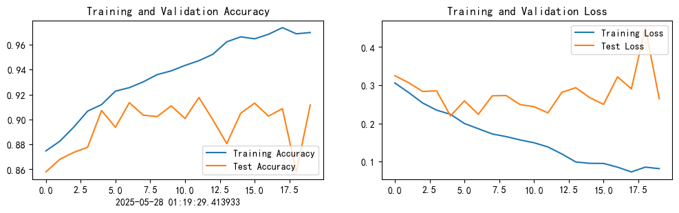
2. 模型评估
#将参数加载到model当中
best_model.load_state_dict(torch.load(PATH, map_location=device))
epoch_test_acc,epoch_test_loss =test(test_dl, best_model, loss_fn)epoch_test_acc,epoch_test_loss(0.917568071615069, 0.22816931214627056)
六、学习心得
1.本周的DenseNet网络模型搭建了DenseLayer模块、DenseBlock模块、Transition模块等。并且应用于乳腺癌病理图像的识别与分类中。DenseLayer模块:每一层接收所有前面层的特征图作为输入,通过批归一化、ReLU、1×1和3×3卷积提取和融合低级与高级特征,增强模型对病理图像中复杂细胞形态的表征能力。DenseBlock模块:由多个DenseLayer堆叠组成,实现层层之间特征的密集连接与融合,有效捕捉乳腺癌病理图像中的多尺度、异质性和细粒度特征。Transition模块:位于DenseBlock之间,通过1×1卷积降维与2×2平均池化下采样压缩特征图尺寸,降低计算复杂度,防止过拟合同时保留关键信息。
2.由于此网络较深,显著增加了内存开销与计算量,代码运行需要耗费大量时间。但是此网络容易达到比较高的准确率。然而,正是这种结构特性,使得DenseNet能够充分提取病理图像中复杂的细粒度特征、核密度、细胞形态与空间结构等重要信息。


 被折叠的 条评论
为什么被折叠?
被折叠的 条评论
为什么被折叠?
 到【灌水乐园】发言


