数据结构与算法(四)

最新推荐文章于 2023-07-15 11:46:41 发布

weixin_42410385

最新推荐文章于 2023-07-15 11:46:41 发布

阅读量311

点赞数

分类专栏：数据结构与算法数据结构

本文链接：https://blog.csdn.net/weixin_42410385/article/details/108661299

版权

数据结构与算法同时被 2 个专栏收录

4 篇文章 0 订阅

订阅专栏

数据结构

4 篇文章 0 订阅

订阅专栏

第四章排序算法

1. 常用算法

根据时间复杂度的不同，主流的排序算法可以分为3大类。

1.1 时间复杂度为 $O(n^2)$ 的排序算法

冒泡排序
选择排序
插入排序
希尔排序（希尔排序比较特殊，它的性能略优于 $O(n^2)$ ，但右比不上 $O (n l o g n)$ ,姑且把它归入本类）

1.2 时间复杂度为 $O (n l o g n)$ 的排序算法

快速排序
归并排序
堆排序

1.3 时间复杂度为线性的排序算法

计数排序
桶排序
基数排序

以上列举的只是最主流的排序算法，在算法界还存在着更多五花八门的排序，它们有些基于传统排序变形而来，有些则是脑洞打开，如鸡尾酒排序、猴子排序、睡眠排序等。
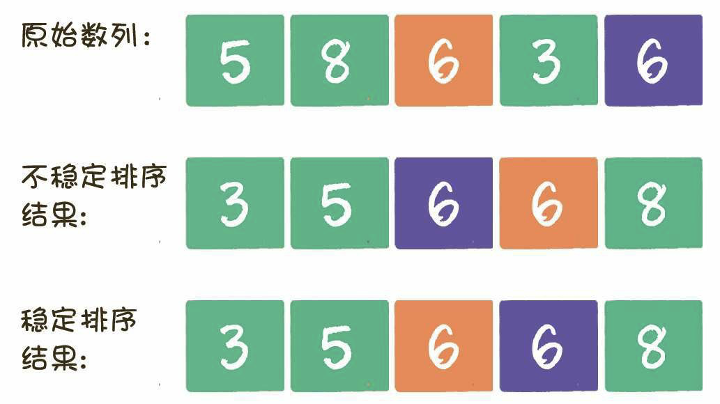
此外，排序算法还可以根据其稳定性，划分为稳定排序和不稳定排序。
既如果值相同的元素在排序后仍然保持着排序前的顺序，则这样的排序算法是稳定排序；如果值相同的元素在排序后打乱了排序前的顺序，则这样的排序算法是不稳定排序。例如下面的例子。

2.什么是冒泡排序

2.1 什么是冒泡排序

冒泡排序是一种稳定排序，值相等的元素并不会打乱原本的顺序。由于该排序算法的每一轮都要遍历所有元素，总共遍历（元素数量-1）轮，所以平均时间复杂度是 $O(n^2)$ 。

    public static void sort1(int[] array) {
        for (int i = 0;i<array.length - 1;i++) {
            for (int j = 0; j < array.length - 1 - i; j++) {
                int temp = 0;
                if (array[j] > array[j+1]) {
                    temp = array[j];
                    array[j] = array[j+1];
                    array[j+1] = temp;
                }
            }
        }
    }

2.1冒泡排序的优化

经过几轮的遍历，有可能整列数据已然是有序的了。可是排序算法仍然兢兢业业地继续执行。在这种情况下，如果能判断出数列已经有序，并做出标记，那么剩下的几轮排序就不必执行了，可以提前结束工作。

/**
     * @Description: 一次优化 
     * 几次轮训结束后 可能已经排好序了，可以结束后面的轮训
     * 
     * @Author: fancg 
     * @Date: 2020/9/18
     **/
    public static void sort2(int[] array) {
        for (int i = 0;i<array.length - 1;i++) {
            boolean isOver = true;
            for (int j = 0; j < array.length - 1 - i; j++) {
                int temp = 0;
                if (array[j] > array[j+1]) {
                    temp = array[j];
                    array[j] = array[j+1];
                    array[j+1] = temp;
                    isOver = false;
                }
            }
            if (isOver)break;
        }
    }

利用布尔变量作为标记。如果在本轮排序中，元素有交换，则说明数列无序；如果没有元素交换，则说明数列已然有序，然后直接跳出大循环。

二次优化主要优化右面元素许多已经是有序的，可以避免没吃多余的比较。

	/**
     * @Description: 二次优化
     * 几次轮训结束后 可能已经排好序了，可以结束后面的轮训
     * 右面的许多元素已经是有序的了，可是每一轮还是白白地比较了许多次，所以可以标记最后一次变更的下标
     * @Author: fancg
     * @Date: 2020/9/18
     **/
    public static void sort3(int[] array) {
        int lastExchangeIndex = 0;
        int sortBorder = array.length - 1;
        for (int i = 0;i<array.length - 1;i++) {
            boolean isOver = true;
            for (int j = 0; j < sortBorder; j++) {
                int temp = 0;
                if (array[j] > array[j+1]) {
                    temp = array[j];
                    array[j] = array[j+1];
                    array[j+1] = temp;
                    isOver = false;
                    lastExchangeIndex = j;
                }
            }
            if (isOver)break;
            sortBorder = lastExchangeIndex;
        }
    }

sortBorder就是无序数列的边界。每一轮排序过程中，处于sortBorder之后的元素就不需要再进行比较了，肯定是有序的。

2.3 鸡尾酒排序

冒泡排序的每一个元素都可以像小气泡一样，根据自身大小，一点一点地向着数组的一侧移动。算法的每一轮都是从左到右来比较元素，进行单向的位置交换的
那么鸡尾酒排序做了怎样的优化呢？
鸡尾酒排序的元素比较和交换过程是双向的。

/**
     * @Description: 鸡尾酒排序
     * 双向排序，一次从前往后，二次从后往前 减少外层循环次数
     * @Author: fancg
     * @Date: 2020/9/18
     **/
    public static void sort4(int[] array) {
        int temp = 0;
        for (int i = 0;i < array.length / 2;i++) {
            boolean isOver = true;
            for (int j = 0; j < array.length - i - 1; j++) {
                if (array[j] > array[j+1]) {
                    temp = array[j];
                    array[j] = array[j+1];
                    array[j+1] = temp;
                    isOver = false;
                }
            }
            if (isOver)break;
            isOver = true;
            for (int j = array.length - i - 1;j > i;j--) {
                if (array[j] < array[j-1]) {
                    temp = array[j];
                    array[j] = array[j-1];
                    array[j-1] = temp;
                    isOver = false;
                }
            }
            if (isOver)break;
        }
    }

3. 什么是快速排序

3.1快速排序

同冒泡排序一样，快速排序也属于交换排序，通过元素之间的比较和交换位置来达到排序的目的。不同的是，冒泡排序在每一轮中只把1个元素冒泡到数列的一端，而快速排序则在每一轮挑选一个基准元素，并让其他比它大的元素移动到数列一边，比它小的元素移动到数列的另一边，从而把数列拆解成两个部分。这种思想就叫做分治法。
在分治法的思想下，原数列在每一轮都被拆分成两部分，每一部分在下一轮又分别被拆分成两部分，直到不可再分为止。
每一轮的比较和交换，需要把数组全部元素都遍历一遍，时间复杂度是 $O (n)$ 。这样的遍历一共需要多少轮呢？假如元素个数是n，那么平均情况下需要logn轮，因此快速排序算法总体的平均时间复杂度是 $O (n l o g n)$ 。

3.2基准元素的选择

基准元素，英文是pivot,在分治过程中，以基准元素为中心，把其他元素移动到它的左右两边。
我们可以随机选择一个元素作为基准元素，并且让基准元素和数列首元素交换位置。
这样一来，即使在数列完全逆序的情况下，也可以有效地将数列分成两部分。
当然，即使是随机选择基准元素，也会有极小的几率选到数列的最大值或最小值，同样会影响分治的效果。
所以，虽然快速排序的平均时间复杂度是 $O (n l o g n)$ ,但最坏情况下的时间复杂度是 $O(n^2)$ 。

3.3 代码实现

/**
 * @author: fancg
 * @create: 2020-09-21
 */
public class QuickSort {

    public static void quickSort(int[] arr,int startIndex, int endIndex) {
        if (startIndex >= endIndex) return;
        int partition = partition(arr, startIndex, endIndex);
        quickSort(arr, startIndex, partition - 1);
        quickSort(arr, partition + 1, endIndex);
    }

    /**
     * @Description: 分治（双边循环法）
     * @Author: fancg
     * @Date: 2020/9/21
     **/
    private static int partition(int[] arr, int startIndex, int endIndex) {
        //取第一个位置（也可以选择随机位置）的元素作为基准元素。
        int pivot = arr[startIndex];
        int left = startIndex;
        int right = endIndex;
        while (left != right) {
            //控制right指针比较向左移
            while (left < right && arr[right] > pivot) {
                right --;
            }
            //控制left指针比较向右移
            while (left < right && arr[left] <= pivot) {
                left ++;
            }
            if (left < right) {
                int i = arr[left];
                arr[left] = arr[right];
                arr[right] = i;
            }
        }
        //pivot 和指针重合点交换
        arr[startIndex] = arr[left];
        arr[left] = pivot;
        return left;
    }

    public static void quickSort2(int[] arr,int startIndex, int endIndex) {
        if (startIndex >= endIndex) return;
        int partition = partition2(arr, startIndex, endIndex);
        quickSort2(arr, startIndex, partition - 1);
        quickSort2(arr, partition + 1, endIndex);
    }

    /**
     * @Description: 非递归实现
     * @Author: fancg
     * @Date: 2020/9/21
     **/
    public static void quickSort3(int[] arr, int startIndex, int endIndex) {
        Stack<Map<String, Integer>> mapStack = new Stack<>();
        Map<String, Integer> map = new HashMap<>();
        map.put("startIndex", startIndex);
        map.put("endIndex", endIndex);
        mapStack.push(map);
        while (!mapStack.isEmpty()) {
            Map<String, Integer> pop = mapStack.pop();
            int partition2 = partition2(arr, pop.get("startIndex"), pop.get("endIndex"));
            if (pop.get("startIndex") < partition2 - 1) {
                Map<String, Integer> left = new HashMap<>();
                left.put("startIndex", pop.get("startIndex"));
                left.put("endIndex", partition2 - 1);
                mapStack.push(left);
            }
            if (partition2 + 1 < pop.get("endIndex")) {
                Map<String, Integer> right = new HashMap<>();
                right.put("startIndex", partition2 + 1);
                right.put("endIndex", pop.get("endIndex"));
                mapStack.push(right);
            }
        }
    }

    /**
     * @Description: 分治（单边循环法）
     * @Author: fancg
     * @Date: 2020/9/21
     **/
    private static int partition2(int[] arr, int startIndex, int endIndex) {
        int pivot = arr[startIndex];
        int mark = startIndex;
        for (int i = startIndex + 1; i <= endIndex; i++) {
            if (arr[i] < pivot) {
                mark++;
                int p = arr[mark];
                arr[mark] = arr[i];
                arr[i] = p;
            }
        }
        arr[startIndex] = arr[mark];
        arr[mark] = pivot;
        return mark;
    }

    public static void main(String[] args) {
    	//双边循环
        int[] ints = {4, 4, 6, 5, 3, 2, 8, 1};
        quickSort(ints, 0, ints.length - 1);
        System.out.println(Arrays.toString(ints));
        //单边循环
        int[] ints2 = {4, 4, 6, 5, 3, 2, 8, 1};
        quickSort2(ints2, 0, ints.length - 1);
        System.out.println(Arrays.toString(ints2));
        //非递归实现
        int[] ints3 = {4, 4, 6, 5, 3, 2, 8, 1};
        quickSort3(ints3, 0, ints.length - 1);
        System.out.println(Arrays.toString(ints3));
    }

4. 什么是堆排序

4.1 传说中的堆排序

二叉堆的特性
1. 最大堆的堆顶是整个堆中的最大元素
2. 最小堆的堆顶是整个堆中的最小元素
堆排序算法的步骤：
1. 把无效数组构建成二叉堆，需要从小到大排序，则构建成最大堆；需要从大到小排序，则构建成最小堆。
2. 循环删除堆顶元素，替换到二叉堆的末尾，调整堆产生新的堆顶。

4.2 堆排序的代码实现

/**
 * 堆排序
 * @author: fancg
 * @create: 2020-09-21
 */
public class HeapSort {

    public static void downAdjust(int[] array, int parentIndex, int length) {
        //temp 保存父节点值，用于最后的赋值
        int temp = array[parentIndex];
        int childIndex = 2 * parentIndex + 1;
        while (childIndex < length) {
            //如果有右孩子，且右孩子的值大于左孩子的值，则定位到右孩子
            if (childIndex + 1 < length && array[childIndex+1] > array[childIndex]) {
                childIndex++;
            }
            if (temp >= array[childIndex])break;
            array[parentIndex] = array[childIndex];
            parentIndex = childIndex;
            childIndex = 2*childIndex+1;
        }
        array[parentIndex] = temp;
        System.out.println(Arrays.toString(array));
    }

    public static void heapSort(int[] array) {
        for (int i = (array.length-2)/2;i>=0;i--) {
            downAdjust(array,i ,array.length);
        }
        for (int i = array.length - 1;i>0;i--) {
            int temp = array[i];
            array[i] = array[0];
            array[0] = temp;
            downAdjust(array, 0 ,i);
        }
    }

    public static void main(String[] args) {
        int[] arr = {1,3,2,6,5,7,8,9,10,0};
        heapSort(arr);
        System.out.println(Arrays.toString(arr));
    }
}

二叉堆的节点下沉调整(downAdjust方法)是堆排序算法的基础，这个调节操作本身的时间复杂度在上一章讲过是 $O (l o g n)$ 。
我们再来回顾一下堆排序算法的步骤。
1. 把无序数组构建成二叉堆。
2. 循环删除堆顶元素，并将该元素移动到集合尾部，调整堆产生新的堆顶。
第一步，把无序数组构建成二叉堆，这一步的时间复杂度是 $O (n)$ 。
第二步，需要进行n-1次循环。每次循环调用一次downAdjust方法，所以第二位的计算规模是 $(n - 1) * l o g n$ ，时间复杂度为 $O (n l o g n)$ 。
两个步骤是并列关系，所以整体的时间复杂度是 $O (n l o g n)$ 。

4.3 堆排序和快速排序对比

堆排序和快速排序的平均时间复杂度都是 $O (n l o g n)$ ,并且都是不稳定排序。至于不同点，快速排序的最坏时间复杂度是 $O(n^2)$ ,而堆排序的最坏时间复杂度稳定在 $O (n l o g n)$ 。
此外，快速排序递归和非排序递归方法的平均空间复杂度都是 $O (l o g n)$ ,而堆排序的空间复杂度是 $O (1)$ 。

5. 计数排序和桶排序

5.1 计数排序

假设数组中有20个随机整数，取值范围为0~10，要求用最快的速度把这20个整数从小到大进行排序。
如何给这些整数进行排序呢？
这些整数只能够在0~10这11个数中取值，取值范围有限。所以可以根据这有限的范围，建立一个长度为11的数组，数组下标从0到10，元素初始值全为0。
遍历时，每一个整数按照其值对号入座，同时对应数组下标的元素进行加一操作。
有了这个统计结果，排序就很简单了。直接遍历数组，输出数组元素的下标值，元素的值是几就输出几次。

/**
 * @author: fancg
 * @create: 2020-09-22
 * 计数排序
 */
public class CountSort {

    public static int[] countSort(int[] array) {
        //得到数列的最大值、最小值
        int max = Arrays.stream(array).max().getAsInt();
        int min = Arrays.stream(array).min().getAsInt();
        //根据数列最大值确定统计数组的长度
        int[] ints = new int[max-min+1];
        //遍历数列，填充统计数组
        for (int i = 0;i<array.length;i++) {
            ints[array[i]]++;
        }
        //遍历统计数组，输出结果
        int index = 0;
        for (int i=0; i<ints.length;i++) {
            for (int j = 0; j < ints[i];j++) {
                array[index++] = i;
            }
        }
        return array;
    }

    public static void main(String[] args) {
        int[] arr = {4,4,6,5,3,2,8,1,7,5,6,0,10};
        countSort(arr);
        System.out.println(Arrays.toString(arr));
    }
}

1. 当数列最大和最小值差距过大时，并不适合用计算排序。
例如给出20个随机整数，范围在0到1亿之间，这时如果使用计数排序，需要创建长度为1亿的数组。不但严重浪费空间，而且时间复杂度也会随之升高。
2. 当数列元素不是整数时，也不适合用计数排序。
如果数列中的元素都是小数，如25.213，或0.00、000、001这样的数字，则无法创建对应的统计数组。这样显然无法进行计数排序。

5.4 什么是桶排序

桶排序同样是一种线性时间的排序算法。类似于计数排序所创建的统计数组，桶排序需要若干个桶来协助排序。
每一个桶(bucket)代表一个区间范围，里面可以承载一个或多个元素。具体需要建立多少个桶，如何确定桶的区间范围，有很多种不同的方式。我们这里创建的桶数量等于原始数列的元素数量，除最后一个桶只包含数列最大值外前面各个桶的区间按照比例来确定。

区间跨度 = （最大值-最小值）/（桶的数量-1）

遍历原始数列，把元素对号入座放入各个桶中。
对每个桶内部的元素分别进行排序。
遍历所有的桶，输出所有元素。


/**
 * @author: fancg
 * @create: 2020-09-22
 * 桶排序
 *
 */
public class BucketSort {

    public static double[] bucketSort(double[] array) {
        //获取最大值、最小值、区间
        double max = Arrays.stream(array).max().getAsDouble();
        double min = Arrays.stream(array).min().getAsDouble();
        double d = (max - min)/(array.length - 1);//区间
        //初始化桶
        List<LinkedList<Double>> bucketSort = new ArrayList<>(array.length);
        for (int i = 0;i < array.length;i++) {
            bucketSort.add(new LinkedList<Double>());
        }
        //遍历原始数组，将每个元素放入桶中
        for (int i = 0;i < array.length;i++) {
            double v = array[i] - min;
            int num = (int) (v / d);
            bucketSort.get(num).add(array[i]);
        }
        //对每个桶内部进行排序
        for (int i = 0;i < bucketSort.size();i++) {
            Collections.sort(bucketSort.get(i));
        }
        //输出全部元素
        double[] doubles = new double[array.length];
        int index = 0;
        for (LinkedList<Double> list : bucketSort) {
            for (double element : list) {
                doubles[index] = element;
                index++;
            }
        }
        return doubles;
    }

    public static void main(String[] args) {
        double[] array = new double[]{4.12,6.421,0.0023,3.0,2.123,8.122,4,12,10.09};
        double[] doubles = bucketSort(array);
        System.out.println(Arrays.toString(doubles));
    }
}

在上述代码中，所有的桶都保存在ArrayList集合中，每个桶都被定义成一个链表（LinkedList）,这样便于尾部插入元素。
同时，上述代码使用了JDK的集合工具类Collections.sort来为桶内部的元素进行排序。Collections.sort底层采用的是归并排序或Timsort,相当于一种时间复杂度为 $O (n l o g n)$ 的排序。
假设原始数列有n个元素，分成n个桶。
下面逐步来分析一下算法复杂度。
第一步，求数列最大、最小值，运算量为n。
第二步，创建空桶，运算量为n。
第三步，把原始数列的元素分配到各个桶中，运算量为n。
第四步，在每个桶内部做排序，在元素分布相对均匀的情况下，所有桶的运算量之和为n。
第五步，输出排序数列，运算量为n。
因此，桶排序的总体时间复杂度为 $O (n)$ 。
空间复杂度同样是 $O (n)$ 。

小结

在这里插入图片描述

weixin_42410385

关注

0
点赞
踩
1

收藏

觉得还不错? 一键收藏
0
评论
数据结构与算法(四)

第四章排序算法 1. 常用算法根据时间复杂度的不同，主流的排序算法可以分为3大类。1.1 时间复杂度为O(n2)O(n^2)O(n2)的排序算法冒泡排序选择排序插入排序希尔排序（希尔排序比较特殊，它的性能略优于O(n2)O(n^2)O(n2)，但右比不上O(nlogn)O(nlogn)O(nlogn),姑且把它归入本类）1.2 时间复杂度为O(nlogn)O(nlogn)O(nlogn)的排序算法快速排序归并排序堆排序1.3 时间复杂度为线性的排序算法计数排序桶.
复制链接

扫一扫