


 本文介绍了ML课程的一个作业,内容涉及使用CNN进行图像分类,重点是数据增强和性能评估。任务包括实现五种图像变换、理解不同的视觉表示,并对比不同基线模型的性能。文章提供了数据下载、预处理方法以及如何利用KaggleAPI。还讨论了预训练模型在不使用权重时的效果,以及如何通过交叉验证和Ensemble提高模型性能。
ML2023Spring - HW3 相关信息:
课程主页
课程视频
Kaggle link
Sample code
HW03 视频
HW03 PDF
个人完整代码分享: GitHub | Gitee | GitCodeP.S. 即便 kaggle 上的时间已经截止,你仍然可以在上面提交和查看分数。但需要注意的是:在 kaggle 截止日期前你应该选择两个结果进行最后的Private评分。
每年的数据集size和feature并不完全相同,但基本一致,过去的代码仍可用于新一年的 Homework。
文章目录
任务目标(图像分类)
使用 CNN 进行图像分类
性能指标(Metric)
在测试集上的分类精度:
A
c
c
=
p
r
e
d
=
=
l
a
b
e
l
l
e
n
(
d
a
t
a
)
∗
100
%
Acc = \frac{pred==label}{len(data)} * 100\% \nonumber
Acc=len(data)pred==label∗100%
数据解析
- ./train (Training set): 图像命名的格式为 “x_y.png”,其中 x 是类别,含有 10,000 张被标记的图像
- ./valid (Valid set): 图像命名的格式为 “x_y.png”,其中 x 是类别,含有 3,643 张被标记的图像
- ./test (Testing set): 图像命名的格式为 “n.png”,n 是 id,含有 3,000 张未标记的图像
数据来源于 food-11 数据集,共有 11 类。
数据下载(kaggle)
To use the Kaggle API, sign up for a Kaggle account at https://www.kaggle.com. Then go to the ‘Account’ tab of your user profile (
https://www.kaggle.com/<username>/account) and select ‘Create API Token’. This will trigger the download ofkaggle.json, a file containing your API credentials. Place this file in the location~/.kaggle/kaggle.json(on Windows in the locationC:\Users\<Windows-username>\.kaggle\kaggle.json- you can check the exact location, sans drive, withecho %HOMEPATH%). You can define a shell environment variableKAGGLE_CONFIG_DIRto change this location to$KAGGLE_CONFIG_DIR/kaggle.json(on Windows it will be%KAGGLE_CONFIG_DIR%\kaggle.json).
gdown 的链接如果挂了或者太慢,可以考虑使用 kaggle 的 api,流程非常简单,替换<username>为你自己的用户名,https://www.kaggle.com/<username>/account,然后点击 Create New API Token,将下载下来的文件放去应该放的位置:
- Mac 和 Linux 放在
~/.kaggle - Windows 放在
C:\Users\<Windows-username>\.kaggle
pip install kaggle
# 你需要先在 Kaggle -> Account -> Create New API Token 中下载 kaggle.json
# mv kaggle.json ~/.kaggle/kaggle.json
kaggle competitions download -c ml2023spring-hw3
unzip ml2023spring-hw3
Gradescope (Report)
from PIL import image什么是 PIL?
PIL (Python Image Library) 是 python 的第三方图像处理库,支持图像存储,显示和处理,能够处理几乎所有的图片格式。
PIL.Image 模块在 sample code 中用于加载图像。
Q1. Augmentation Implementation
需要完成至少 5 种 transform,这一步能让你熟悉 Data Augmentation 到底是在做什么。
直接看代码部分,调用了 transforms 中的函数。
往回追溯:
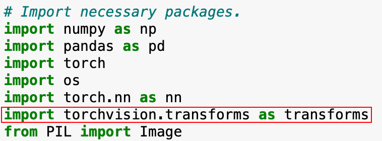
可以看到 transforms 其实就是 torchvision.transforms。
torchvision.transforms 是 pytorch 中的图像预处理包,提供了常用的图像变换方式,可以通过 Compose 将多个变换步骤整合到一起,你可以查看这篇文章:torchvision.transforms 常用方法解析(含图例代码以及参数解释)进一步了解,最好是自行组合 5 个跑几次实验之后再偷懒。
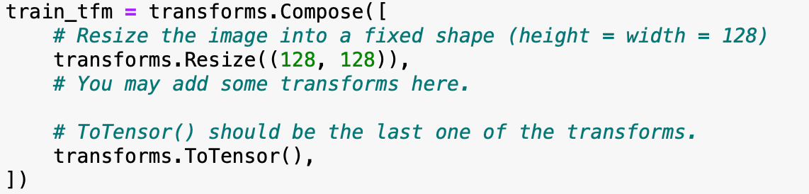
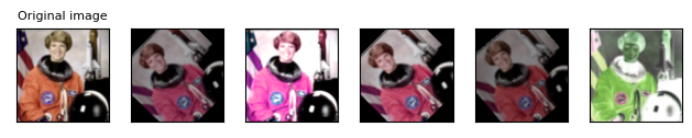
下面的代码可以让你看到 train_tfm 究竟做了什么变换。
# I want to show you an example code of Q1. Augmentation Implementation that visualizes the effects of different image transformations.
import matplotlib.pyplot as plt

plt.rcParams["savefig.bbox"] = 'tight'

# You can change the file path to match your image
orig_img = Image.open('Q1/assets/astronaut.jpg')


def plot(imgs, with_orig=True, row_title=None, **imshow_kwargs):
    if not isinstance(imgs[0], list):
        # Make a 2d grid even if there's just 1 row
        imgs = [imgs]

    num_rows = len(imgs)
    num_cols = len(imgs[0]) + with_orig
    fig, axs = plt.subplots(nrows=num_rows, ncols=num_cols, squeeze=False)
    for row_idx, row in enumerate(imgs):
        row = [orig_img] + row if with_orig else row
        for col_idx, img in enumerate(row):
            ax = axs[row_idx, col_idx]
            ax.imshow(np.asarray(img), **imshow_kwargs)
            ax.set(xticklabels=[], yticklabels=[], xticks=[], yticks=[])

    if with_orig:
        axs[0, 0].set(title='Original image')
        axs[0, 0].title.set_size(8)
    if row_title is not None:
        for row_idx in range(num_rows):
            axs[row_idx, 0].set(ylabel=row_title[row_idx])

    plt.tight_layout()

# Create a list of five transformed images from the original image using the train_tfm function
demo = [train_tfm(orig_img) for i in range(5)]

# Convert the transformed images from tensors to PIL images
pil_img_demo = [Image.fromarray(np.moveaxis(img.numpy()*255, 0, -1).astype(np.uint8)) for img in demo]

# Plot the transformed images using the plot function
plot(pil_img_demo)
Q2. Visual Representations Implementation
下图是 Top/Mid/Bottom 的定义,你可以在 sample code 的最下面找到完成这个问题的代码。
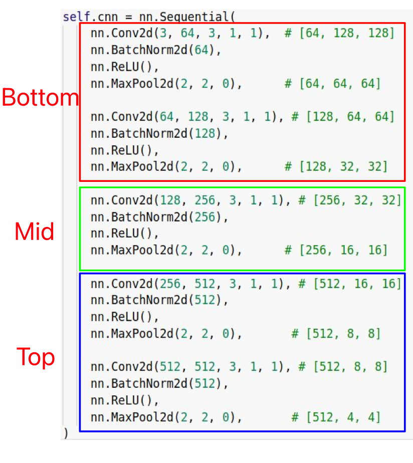
根据你的模型修改其中的 index。
Baselines
为了方便理解,我将原文件重新分为了三部分: Medium,Strong,Boss,每一个都可以独立运行,并相应的达成 baseline,你可以查看这些文件来帮助自己更好的掌握知识。
Simple baseline (0.637)
- 运行所给的 sample code
Medium baseline (0.700)
-
做数据增强
RandomChoice 很好用,另外,lamda x:x 可以返回原图。
-
训练更长时间
根据 PDF 给出的参考训练时间,simple 是 0.5h,medium 是 1.5h,那么在这里我选择的是简单的将原来的 epoch *= 3,也就是 24 个 epoch 来进行最终的训练
Strong baseline (0.814)
-
使用预训练模型
这里你可能有疑惑:不是说不能使用预训练模型吗?
是的,你只能使用预训练模型的架构,不能使用预训练的权重,下面是不使用权重的参数设置。- Torchvision 版本 < 0.13 -> pretrained=False
- > 0.13 -> weights=None
模型对比 (160 epoch, 10 patience, ReduceLROnPlateau,使用了相当于原数据20倍的transforms,单纯修改最后一层的输出维度为 11) :
- 初始模型:0.80000
- resnet50: 0.732
- vgg16: 0.64733
- densenet121: 0.76533
- alexnet: 0.61866
- squeezenet: 0.64200
我觉得这一项的主要目的在于让你认识这些预训练模型的架构,因为可以看到,不使用预训练参数的情况下,实验结果并没有变得更好(使用预训练参数的话,以resnet50为例,仅使用预训练模型就可以轻松到达strong baseline,你可以试试,但不要用它来当作你的kaggle结果)。
但既然PDF中的hint仅仅只是使用预训练模型,我相信一定有什么地方可以调优,使得仅使用预训练模型架构就可以达到 strong baseline,简单对比了使用参数和不使用参数的情况下 acc 的提升情况,发现同样的 lr,使用预训练参数的时候上升幅度更大,所以我想了下:
- 有没有可能是我的 lr 太小了?调大试试
- 会不会是我的transforms不够,因为在我的代码中,5%的可能性不进行transforms,也就是说,20倍的数据增强。50倍试试
- Medium baseline的工作没做好,加TTA(Test Time Augmentation),将train_tfm用到测试集上试试
但上述方法都没有得到好的效果,最终我直接用最开始的CNN模型跑了200多个epoch完成了该strong baseline。
PS:可以将残差和的思想用于模型架构中提升基础性能

因为佛系更新,所以我开始慢慢打磨之前的代码文件 😃
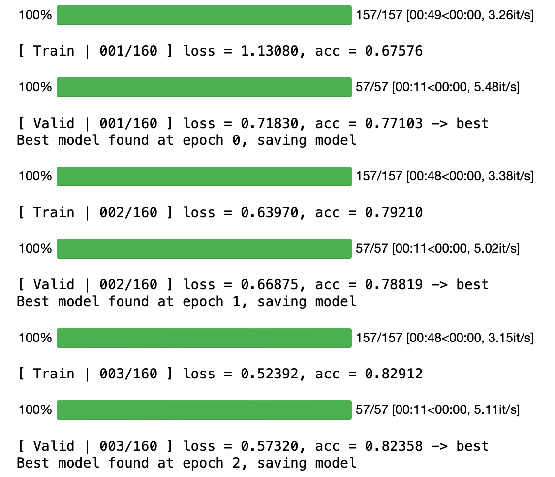
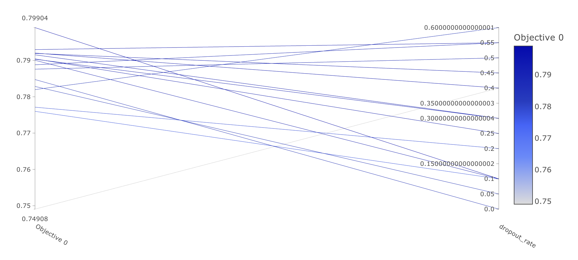
我在代码的全连接层增加了 dropout,并跑了一些实验(100 个 epoch)来寻找较好的 dropout_rate,简单分享一下,也许可以节省你的时间。
对应的 kaggle 得分:
dropout_rate public_score private_score 0 0.78466 0.79266 0.1 0.78800 0.79266 0.2 0.78400 0.78333 0.25 0.80866 0.79666 0.3 0.79866 0.81666 0.4 0.79000 0.79466 0.45 0.78866 0.79800 0.5 0.81666 0.80000 0.55 0.79533 0.79000 0.6 0.77733 0.78466 仅从 public_score 考虑,接下来都片面的选择 dropout_rate=0.5。
可以看到,在仅增加 dropout 层的时候,100个epoch便能达成strong baseline,虽然很勉强,但参考时间所对应的 epoch 是大于等于 160 的,所以在此便已经完成了目标。
注意一下,预训练模型直接使用:self.cnn = nn.Sequential(list(resnet50(weights=None).children())[:]) 后再加全连接层的话会出 shape 不匹配的错误,应该使用 self.cnn = nn.Sequential(list(resnet50(weights=None).children())[:-1]) 后 flatten 处理再接全连接层,这里说起来可能不直观,可以去代码中理解,如果你不需要完成 Q2,那不赋值给 cnn 一样可以。
Boss baseline (0.874)
-
Cross validation 交叉验证
-
Ensemble 模型集合
相关视频: ML Lecture 22: Ensemble ,如果没有科学上网,这里是两个相同视频的链接地址:bilibili,学校官网。关于stacking,这里有两个非常不错的链接供你学习:Kaggle机器学习之模型融合(stacking)心得,Introduction to Ensembling/Stacking in Python
但其中的细节对于当前的 hw 来说其实有一些问题,不能直接搬运。
- 有一件事困惑了我很久,在做 stacking 的时候,为了严谨,我检查了同个模型跑出来的结果,然后发现导入相同的模型跑出来的结果竟然不相同,将代码精简后也无果,最后我检查发现,是因为 train_tfm 让其每次的输入都不同 😦
那问题就明了了,可以将 kfold 分出的 valid_set 用 test_tfm 来固定它,具体实现:重写 subset 类,传入 tfm 决定使用哪种 transform。
在做完 CV 和 stacking 后,kaggle 的分数卡在了 0.85333,有一个提升方法是在 strong baseline 下修改 Classifier 的架构以获得更好的初始结果。
不知道是否是我的原因,但 TTA 在此处的提升不大。
下表是各模型在 epoch=200, patience=20, dataset=merge 下的 kaggle 分数,& 表示stacking。
model publicScore privateScore Classifier & ResNet50 & DenseNet121 0.85333 0.84200 Classifier 0.84200 0.83133 Classifier & DenseNet121 0.83866 0.83333 ResNet50 & DenseNet121 0.83666 0.82466 DenseNet121 0.83666 0.83133 Classifier & ResNet50 0.83400 0.82066 ResNet50 0.82600 0.81000 - 有一件事困惑了我很久,在做 stacking 的时候,为了严谨,我检查了同个模型跑出来的结果,然后发现导入相同的模型跑出来的结果竟然不相同,将代码精简后也无果,最后我检查发现,是因为 train_tfm 让其每次的输入都不同 😦
小坑
- 注意你的 lr,我在做 cross validation 的时候,不小心将 lr 设置的过大,导致一开始学习的很差,还以为是数据集划分的索引问题,折腾了半天。
- 如果你将
train文件夹和valid文件夹下的内容合并成一个新的文件夹(为了做 cross validation),那么在做 K-fold 的时候,序号一定要 shuffle 去打乱,你只要默认打乱了,就不需要考虑太多,否则就会出现一种情况:验证集的标签有可能在训练集中不存在,那就意味着,你的模型可能几乎没见过验证集里面的 label,如果完全没见过,那 acc 甚至有可能是 0。下面是我当时疏忽导致的 bug: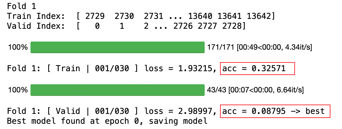


 4973
4973

 被折叠的 条评论
为什么被折叠?
被折叠的 条评论
为什么被折叠?
 到【灌水乐园】发言


