


1. 前言
经典永不过时。这篇文章中,我们要回顾卷积神经网络发展史上几个经典模型:LeNet、AlexNet、NiN、VGGNet、ResNet,梳理它们的发展脉络,总结它们各自的特点,并借助Pytorch完成实现。
2. 模型及实现
2.1 LeNet
LeNet是LeCun在1998年提出的用于解决手写数字识别任务的卷积神经网络模型,这一网络模型奠定了之后CNN的基本架构。它又被称为LeNet-5,5表示第5代版本。LeNet-5的基本结构是:卷积、池化、卷积、池化、全连接。
LeNet-5网络结构如下图:
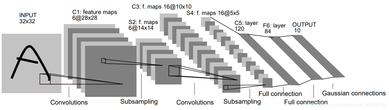
LeNet的主要贡献:奠定了之后的CNN架构,无论何种CNN模型都逃不出卷积/池化/全连接(非线性激活函数)的基本模式,标志着卷积神经网络时代的到来。
代码实现
import torch.nn as nn
import torch.nn.functional as F

class LeNet(nn.Module):
    def __init__(self, num_class):
        super(LeNet, self).__init__()
        self.conv1 = nn.Conv2d(3, 16, (5,5), 1)
        self.pool = nn.MaxPool2d(2, 2)
        self.conv2 = nn.Conv2d(16, 32, (5,5), 1)
        self.fc1 = nn.Linear(32*5*5, 120)
        self.fc2 = nn.Linear(120, 84)
        self.fc3 = nn.Linear(84, num_class)

    def forward(self, x):
        x = self.pool(self.conv1(x))
        x = self.pool(self.conv2(x))
        x = x.view(-1, 32*5*5)
        x = F.relu(self.fc1(x))
        x = F.relu(self.fc2(x))
        x = self.fc3(x)
        return x
2.2 AlexNet
LeNet在早期的小规模数据集上表现还不错,一些机器学习方法(支持向量机等)也能与之掰掰手腕。LeNet面临的主要问题是神经网络的深度不够,这受限于当时的硬件条件。2000年后,通用GPU的概念被提出。GPU擅长矩阵计算,最初的用途是计算机图形学的相关计算。2010年后,GPU开始被广泛用在机器学习领域。2012年,Alex Krizhevsky提出了AlexNet,凭借top5-15.3%的误差率在当年ImageNet图像分类大赛获得冠军。从这一年开始,卷积网络的深度越来越深。AlexNet的深度为8层,包括:5个卷积层,3个全连接层。
AlexNet的网络结构如下图所示:
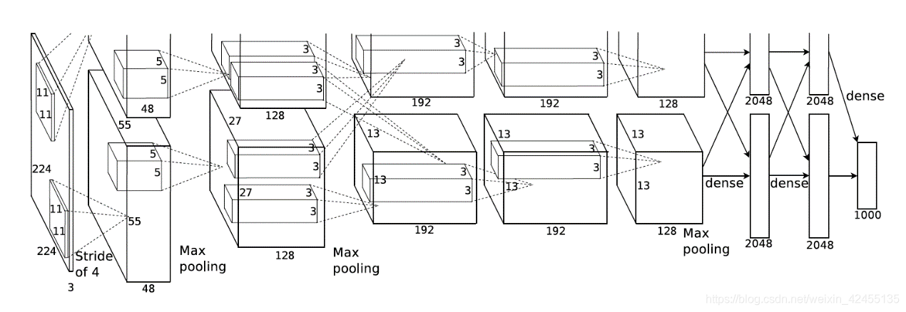
值得注意的是作者Alex采取了两块GPU来训练,因此出现了上图中两个“并行的”计算过程。两块GPU的计算同时进行,整体上实现了特征图通道数加倍的效果。以第一层为例:输入图片尺寸为224x224x3,分别经过上下5x5x48的卷积核后得到55x55x48的特征图,因此这一层的输出特征图尺寸为55x55x96.因为现在计算条件比以前好太多,我们在实现AlexNet的时候不需要分两块GPU计算,直接选择5x5x96的卷积核即可。不过,这个思路值得学习。
AlexNet的主要贡献:1)从此卷积神经网络步入深度卷积网络时代。2)提供了很多训练技巧:多GPU加速训练,数据增强提升泛化能力,Dropout防止过拟合等。
import torch.nn as nn

class AlexNet(nn.Module):
    def __init__(self, num_class):
        super(AlexNet, self).__init__()
        self.conv1 = nn.Sequential(
            nn.Conv2d(3, 96, (11, 11), 4, 2), # 224x224x3 -> 55x55x96
            nn.ReLU(inplace=True),
            nn.MaxPool2d(3, 2) # 27x27x48
        )
        self.conv2 = nn.Sequential(
            nn.Conv2d(96, 256, (5, 5), 1, 2), # 27x27x256
            nn.ReLU(inplace=True),
            nn.MaxPool2d(3, 2) # 13x13x128
        )
        self.conv3 = nn.Sequential(
            nn.Conv2d(256, 384, (3, 3), 1, 1), # 13x13x384
            nn.ReLU(inplace=True),
        )
        self.conv4 = nn.Sequential(
            nn.Conv2d(384, 384, (3, 3), 1, 1), # 13x13x384
            nn.ReLU(inplace=True)
        )
        self.conv5 = nn.Sequential(
            nn.Conv2d(384, 256, 3, 1, 1), # 13x13x256
            nn.ReLU(inplace=True),
            nn.MaxPool2d(3, 2) # 6x6x256
        )
        self.fc1 = nn.Sequential(
            nn.Linear(6*6*256, 4096), # 4096
            nn.ReLU(),
            nn.Dropout(0.5)
        )
        self.fc2 = nn.Sequential(
            nn.Linear(4096, 4096), # 4096
            nn.ReLU(),
            nn.Dropout(0.5)
        )
        self.fc3 = nn.Linear(4096, num_class)

    def forward(self, x):
        x = self.conv1(x)
        x = self.conv2(x)
        x = self.conv3(x)
        x = self.conv4(x)
        x = self.conv5(x)
        x = x.view(-1, 6*6*256)
        x = self.fc1(x)
        x = self.fc2(x)
        x = self.fc3(x)
        return x
2.3 NiN
2013年末,ICLR接收了来自NUS的这篇《Network In Network》。本文提出的NiN模型在结构上大胆创新,超越了当年的SOTA。
NiN的创新体现在两方面:1.采用多层感知器(MLPconv)代替传统卷积,取得了很好的效果;2.采用全局平均池化(GAP)来代替传统全连接层,从而实现抗过拟合。NiN网络的整体架构图如下:
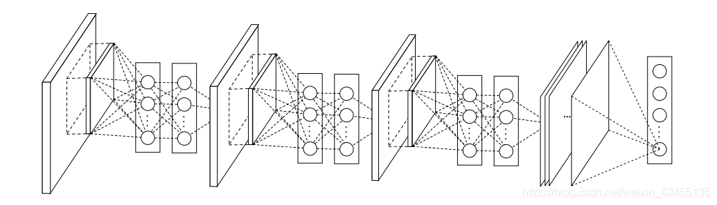
所谓多层感知器,就是在已有的卷积层后多加了1x1卷积,这1x1卷积后续被证明是很有效的。一方面1x1卷积可以在不改变特征图长宽的情况下改变通道数,并可以大幅度减少参数数量,另一方面1x1卷积也显著提升了卷积层提取特征的能力。全局平均池化如图所示:将特征图的一个通道的全局平均作为某个输出节点的置信度。这样一来,就摆脱了全连接层广受诟病的“黑盒模式”,增强了网络的可解释性。但是也带来了问题:模型更难迁移和训练。GAP只能说是结构上的一次大胆尝试,并没有撼动全连接层的地位。总体来说,NiN某种程度上是把原本处于最后一层的全连接层给提前到了前面的卷积层中,从而增强了CNN提取特征的能力。
NiN的主要贡献:首次提出1x1卷积,为后续许多网络模型借鉴。
代码实现
import torch
import torch.nn as nn

class NIN(nn.Module):
    def __init__(self):
        super(NIN, self).__init__()
        self.layer = nn.Sequential(
            nn.Conv2d(3, 192, 5, 1, 2),
            nn.ReLU(inplace=True),
            nn.Conv2d(192, 160, 1),
            nn.ReLU(inplace=True),
            nn.Conv2d(160, 96, 1),
            nn.ReLU(inplace=True),
            nn.MaxPool2d(3, 2, 1),
            nn.Dropout(0.5),

            nn.Conv2d(96, 192, 5, 1, 2),
            nn.ReLU(inplace=True),
            nn.Conv2d(192, 192, 1),
            nn.ReLU(inplace=True),
            nn.Conv2d(192, 192, 1),
            nn.ReLU(inplace=True),
            nn.MaxPool2d(3, 2, 1),
            nn.Dropout(0.5),

            nn.Conv2d(192, 192, 3, 1, 1),
            nn.ReLU(inplace=True),
            nn.Conv2d(192, 192, 1),
            nn.ReLU(inplace=True),
            nn.Conv2d(192, 10, 1),
            nn.ReLU(inplace=True),
            nn.AvgPool2d(8, 1),
        )

    def forward(self, x):
        out = self.layer(x)
        out = torch.flatten(out, 1)
        return out
2.4 VGG
AlexNet引领卷积神经网络朝深度越来越深的方向发展。在2014年,牛津大学VGG组在提出了VGG,并凭借此模型取得了ILSVRC 2014比赛分类项目的第二名(第一名是GoogLeNet)。VGG相对AlexNet的深度更深,卷积核更小(3x3)。
VGG有6个变体,是根据网络层数的不同来划分的,如下图所示:
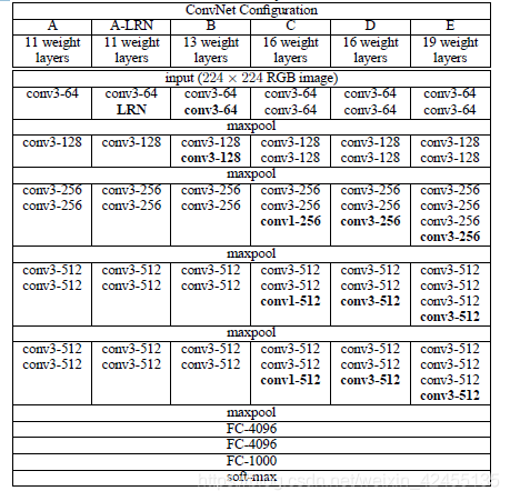
观察VGG网络结构,整体上可以分为6个模块,前5个模块都是卷积操作,最后1个模块是全连接操作。在卷积时,VGG广泛采用了kernel_size=3,stride=1,padding=1和kernel_size=1,stride=1,padding=0的卷积核,这种卷积核不改变特征图的尺寸,只改变通道数;在池化时,VGG采用kernel_size=2,stride=2,每轮池化使得特征图尺寸缩小1/2,经过5轮池化,特征图尺寸变为224/32=7。
对比VGG的变体的不同:A版本是最初级的,又名VGG-11;A-LRN版本在A的基础上引入了LRN,但实验结果表明没啥效果;B版本比A版本增加2个3x3卷积层;C版本比B版本增加了3个1x1卷积层;D版本将C版本增加的1x1卷积换成3x3卷积,成为了经典的VGG-16;E版本又增加了3个3x3卷积层。
总结起来,VGG的显著特点就是:用重复的小型卷积层堆叠深度。随着深度的增加,卷积网络也变得越来越不好训练。对于解决深度卷积网络参数初始化问题,在论文中,研究人员采用了Pre-training的方法:先在VGG的A版本网络上训练,得到稳定的效果后逐步加深卷积层深度。
VGG的主要贡献:验证了加深深度确实可以提升卷积神经网络性能,但发现逐渐遇到瓶颈。验证了堆积小卷积核的性能优于大卷积核(7x7,11x11)的性能。
代码实现
import torch.nn as nn

def vgg_blocks(params):
    layers = []
    in_channel = 3
    for p in params:
        if p == 'M':
            layers += [nn.MaxPool2d(2, 2)]
        else:
            layers += [nn.Conv2d(in_channel, p, kernel_size=3, stride=1), nn.ReLU()]
            in_channel = p
    return nn.Sequential(*layers)

class VGG(nn.Module):
    def __init__(self, params, num_class=1000):
        super(VGG, self).__init__()
        self.vgg_conv = vgg_blocks(params)
        self.fc = nn.Sequential(
            nn.Linear(7*7*512, 4096),
            nn.ReLU(),
            nn.Dropout(0.5),
            nn.Linear(4096, 4096),
            nn.ReLU(),
            nn.Dropout(0.5),
            nn.Linear(4096, num_class)
        )

    def forward(self, x):
        x = self.vgg_conv(x)
        x = self.fc(x)
        return x

vgg_16 = [64, 64, 'M', 128, 128, 'M', 256, 256, 'M', 512, 512, 'M', 512, 512, 'M']
net = VGG(vgg_16, 1000)
2.5 ResNet
何恺明在2015年提出ResNet,一举获得了ILSVRC2015分类任务的第一名和CVPR2016最佳论文。ResNet使得训练百层甚至千层的神经网络成为可能,毫无疑问地成为了计算机视觉领域的里程碑。
自从AlexNet开始,后续的网络模型的深度开始向越来越深的方向发展。但是,随着模型深度的增加,模型的表现反而会变差。通常,我们认为这是因为梯度消失/爆炸导致的。为此解决这一问题,人们创造了一系列遏制梯度消失/梯度爆炸的方法,例如:预训练、权重初始化(Normalized Initialization)、中间归一化层(BN、LN等)、正则化、ReLU等等。何恺明也在论文中说:梯度消失/爆炸这个问题已经被解决得差不多了。那么ResNet解决了什么问题呢?
要回答这个问题,我们需要理解ResNet的核心结构:“短接”(short-cut)。“短接”让网络模型自行决定模型的深度。ResNet的“短接”结构如下图所示:
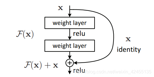
从本质上理解短接结构或许需要一些微分方程、流形几何之类的数学知识,这里我们可以直觉一点来尝试理解。在反向传播的过程中,由于 ,所以
,所以 ,可以看到右边式子展开必有1,这意味着梯度可以一直传播到很前面的层。这里其实也顺便解决了深度网络模型的梯度消失/爆炸问题。然而这个结构的效果不仅于此,深度网络模型的一个问题就是:它很难拟合恒等映射,即拟合H(x)=x。但是,添加了“短接”操作就可以拟合了。当F(x)→0时,H(x)=x+F(x)→x。这就意味着,ResNet可以自行地决定哪些层“被短接“。
ResNet的5个版本如下表所示:
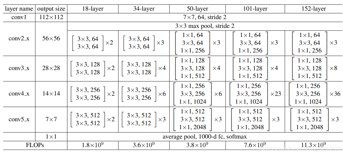
在具体实现上,不同版本的ResNet除了层数不同外,在基本模块的设计上也存在差异。18-layer、34-layer的基本模块称为“BasicBlock”,由2个3x3卷积(kernel_size=3,stride=1,padding=1)组成,short-cut部分采用identity;50-layer、101-layer、152-layer的基本模块称为“Bottleneck”,由1x1卷积、3x3卷积、1x1卷积组成,short-cut部分可采用identity和1x1卷积。
ResNet的主要贡献:通过提出残差结构,较好地解决了网络深度增加时性能下降的问题,使得训练深层网络成为可能。
代码实现
import torch
import torch.nn as nn

def conv3x3(in_channels, out_channels):
    return nn.Sequential(
        nn.Conv2d(in_channels, out_channels, 3, 1, 1),
        nn.BatchNorm2d(out_channels),
    )

def conv1x1(in_channels, out_channels):
    return nn.Sequential(
        nn.Conv2d(in_channels, out_channels, 1, 1),
        nn.BatchNorm2d(out_channels),
    )

class BasicNet(nn.Module):
    def __int__(self, in_channel, out_channel, downsample=None):
        super(BasicNet, self).__init__()
        self.conv1 = conv3x3(in_channel, out_channel)
        self.conv2 = conv3x3(out_channel, out_channel)
        self.relu = nn.ReLU(inplace=True)
        self.downsample = downsample

    def forward(self, x):
        identity = x
        out = self.conv1(x)
        out = self.relu(out)
        out = self.conv2(out)
        out = self.relu(out)
        if self.downsample is not None:
            identity = self.downsample(x)
        out += x
        out = self.relu(out)
        return out

class BottleNet(nn.Module):
    def __init__(self, in_channel, out_channel, extension=4, downsample=None):
        super(BottleNet, self).__init__()
        self.extension = extension
        self.downsample = downsample
        self.conv1 = conv1x1(in_channel, out_channel)
        self.conv2 = conv3x3(out_channel, out_channel)
        self.conv3 = conv1x1(out_channel, self.extension * out_channel)
        self.relu = nn.ReLU(inplace=True)

    def forward(self, x):
        identity = x
        out = self.conv1(x)
        out = self.relu(out)
        out = self.conv2(out)
        out = self.relu(out)
        out = self.conv3(out)
        if self.downsample is not None:
            identity = self.downsample(x)
        out = out + identity
        out = self.relu(out)
        return out

class ResNet50(nn.Module):
    def __init__(self, block, cnt, extension=4):
        super(ResNet50, self).__init__()
        self.pool1 = nn.MaxPool2d(2, 2)
        self.pool2 = nn.MaxPool2d(3, 2)
        self.relu = nn.ReLU(inplace=True)
        self.extension = extension
        self.conv1 = nn.Conv2d(3, 64, kernel_size=7, stride=2, padding=3)
        self.layer1 = self._make_layers(block, 64, 64, cnt[0])
        self.layer2 = self._make_layers(block, 256, 128, cnt[1])
        self.layer3 = self._make_layers(block, 512, 256, cnt[2])
        self.layer4 = self._make_layers(block, 1024, 512, cnt[3])
        self.pool3 = nn.AvgPool2d(7 * 7 * 2048)
        self.fc = nn.Linear(7*7*2048, 1000)

    def forward(self, x):
        out = self.conv1(x)
        out = self.pool2(out)
        out = self.relu(out)
        out = self.layer1(out)
        out = self.pool1(out)
        out = self.layer2(out)
        out = self.pool1(out)
        out = self.layer3(out)
        out = self.pool1(out)
        out = self.layer4(out)
        out = self.pool1(out)
        out = self.pool3(out)
        out = out.view(x.shape[0], -1)
        out = self.fc(out)
        return out

    def _make_layers(self, block, inc, outc, cnt):
        layers = []
        layers.append(block(inc, outc))
        for i in range(cnt - 1):
            layers.append(block(outc*self.extension, outc))
        return nn.Sequential(*layers)

cnts = [3, 4, 6, 3]
resnet = ResNet50(BottleNet, cnts, 4)
3. 总结
LeNet作为卷积神经网络的开篇,奠定了CNN基本结构;AlexNet尝试加深网络,进入深度卷积神经网络时代,为解决深度网络模型中难以训练、梯度爆炸/消失的问题,提出一系列技巧,如多GPU并行计算、数据增强、Dropout等;NIN、VGG发现小卷积核具有较好的表现,但仍旧无法突破瓶颈;ResNet较好地解决了深度网络模型精度下降的问题,标志着训练深度模型成为可能。
时至今日,算力不断提升,数据不断增加,网络结构不断改进,然而神经网络对于人们来说仍然是个黑盒。经验主义的构造或许并不能给我们带来真正的进步,期待神经网络界“牛顿”的到来!
4. 参考文献
[1] Lecun Y , Bottou L . Gradient-based learning applied to document recognition[J]. Proceedings of the IEEE, 1998, 86(11):2278-2324.
[2] Krizhevsky A , Sutskever I , Hinton G . ImageNet Classification with Deep Convolutional Neural Networks[C]// NIPS. Curran Associates Inc. 2012.
[3] Simonyan K , Zisserman A . Very Deep Convolutional Networks for Large-Scale Image Recognition[J]. Computer Science, 2014.
[4] M. Lin, Q. Chen, and S. Yan. Network in network. ICLR,2014. 3, 5
[5] K. He, X. Zhang, S. Ren, and J. Sun. Deep residual learning for image recognition. Computer Vision on Pattern Recognition, pages 770–778, 2016.


 被折叠的 条评论
为什么被折叠?
被折叠的 条评论
为什么被折叠?
 到【灌水乐园】发言


