Quantum-Lazy-Learning(量子懒惰学习)详解

Background

近些年来，量子机器学习算法不断地涌现出来，这些算法大部分以张量网络为桥梁，可以来处理计算机视觉、模式识别以及自然语言处理等领域的问题[1-8]。其中一大类算法是采用量子态空间来表示样本的概率分布，从而完成生成或分类的任务【6】。 Quantum Lazy Learing就是其中一种，不过它并不是一种受欢迎的量子机器学习分类算法，它在论文中常以各种各样的形式出现并被摒弃，但它好在具有简单的形式，易于理解。在B站视频《张量网络基础课程》的第23小节对lazy learning做了详细的阐述，它在mnist上的分类达到97%之高。感兴趣的同学还可以结合视频中提到的论文GTNC【6】进行进一步的了解，下面将详细介绍它的内容。

Content

lazy learning基于等概率假设，该假设内容是：所有训练样本在量子态空间出现的概率相同。这样将不同的样本映射到量子态空间后，就会自然的形成一个个聚类。以mnist举例来说，映射后的样本在Hilbert空间中会自然的形成十个簇。那么当我们试图对一张新的图片分类时，只需要求出该样本表示的量子态与不同数字簇的距离，用argmax函数即可求得样本的分类结果（属于哪个数字簇）。不同于我们常用的欧式距离，这里我们采用保真度来衡量两个量子态的相似性。不同距离度量对分类效果的差异可以详细参考上面提到的GTNC [6]。

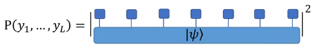
对于具备$L$个像素的图片集而言（或具备$L$个特征量的样本集），我们假设其联合概率分布由$L$个qubit构成的多体态（记为$|\phi ⟩$）描述，满足
$$\mathrm{P}\left(y_1,\dots ,y_L\right)={\left(\prod _{\otimes l=1}^L\left|⟨y_l\mid \psi ⟩\right|\right)}^2$$
$P(y_1,...,y_L)$表示该概率分布给出的样本$Y=(y_1,...,y_L)$出现的概率，用图形表示为

由此可见，只需要知道训练集，即可通过特征映射计算出${\phi }^{lazy}$态，而不包含任何训练和更新过程，${\phi }^{lazy}$态也不包含任何变分参数，因此通过这种方式进行分类监督学习任务被称为量子懒惰学习(quantum lazy learning)，唯一的超参数就是映射函数的选择，可以是$(x,1-x)$、$(\sqrt{x},\sqrt{1-x})$或者是$(sin(\frac{\pi }{2}{x}_i),cos(\frac{\pi }{2}{x}_j))$【10】等等。

以mnist为例，对于不同的数字可以定义10个lazy态
$$|{\phi }_k^{lazy}⟩=\frac{1}{\sqrt{|\mathbb{X}|}\mid }\sum _{X\in {\mathbb{X}}_k}\prod _{\otimes l=1}^L|x_i⟩$$
同时这样的lazy态满足概率归一条件
$$⟨{\psi }^{\text{lazy }}\mid {\psi }^{\text{lazy }}⟩=\frac{1}{|x|}\sum _{X,X^{\prime }\propto x}⟨X\mid X^{\prime }⟩\approx \frac{1}{|x|}\sum _{X,X^{\prime }\propto x}{\delta }_{X,X^{\prime }}=1$$
当然由于式中的累乘，使得量子态的表示是指数复杂的，以mnist为例，需要$2^{784}$(特征映射维度为2时)的空间来表示，这对经典计算机显然是一个不可能任务。因此在实际计算时，可以将样本与lazy态的内积化简到多项式级别复杂度进行计算，下面对该方式进行进一步的讨论。

Supplementary

上面我们提到lazy态的表示为
$$|{\phi }_k^{lazy}⟩=\frac{1}{\sqrt{|\mathbb{X}|}\mid }\sum _{X\in {\mathbb{X}}_k}\prod _{\otimes l=1}^L|x_i⟩$$
对于样本$|Y⟩={\prod }_{\otimes l=1}^L|s_i⟩$，样本在lazy态中的概率(保真度)表示为
$$\begin{gathered} P_k(Y)={\left|⟨Y^{\ast }\mid {\psi }_k^{\mathrm{lazy}}⟩\right|}^2 \\ =\frac{1}{|\mathbb{X}|}\cdot \mid \sum _{\mathrm{X}\in {\mathbb{X}}_{\mathrm{k}}}\prod _{\otimes l=1}^L⟨S_l\mid x_l⟩{|}^2 \end{gathered}$$
从这个结果的角度来分析，通过这样的转换的确是将避免了直接表示lazy态的指数复杂度$O(d^L)$，将其降为多项式计算复杂度$O(NLd)$。但这样运算导致的一个后果就是当样本$Y$和训练集样本$X$一旦有一个像素不同，那么累乘的概率就必定为0。即使将其表示为灰度图片，那么累乘也会使得该运算的结果指数小，求得的概率也就没有意义。

这一点在咨询了首师大的冉老师之后得到解决。在他最新的工作【9】中，样本表示的指数小问题被重新拿出来分析。作者的做法是采用对数保真度来转化累乘，同时引入了$ϵ$偏置项来保证模型的稳定。于是上述公式也可以被描述为
$$\begin{gathered} P_k(Y)=\frac{1}{|\mathbb{X}|}\cdot \mid \sum _{\mathrm{X}\in {\mathbb{X}}_{\mathrm{k}}}\prod _{\otimes l=1}^L⟨S_l\mid x_l⟩{|}^2 \\ =\frac{1}{|\mathbb{X}|}\cdot \mid \sum _{\mathrm{X}\in {\mathbb{X}}_{\mathrm{k}}}\sum _{l=1}^{L}lo{g}_{10}(⟨S_l\mid x_l⟩+ϵ){|}^2 \end{gathered}$$
其中$ϵ$是一个接近0的很小的数，是为了避免出现$log0$的情况。这样使得样本间概率指数衰减的问题就得到解决。下一部分将展示lazy learning的核心代码供大家学习，与上述公式所描述的过程是一致的。

Code

下面是将lazy learning用于mnist数据集图像分类的一个例子，仅给出了核心代码，同时写了一些注释供大家参考学习。

def lazy_learning(train_images, test_images, mode = 'mapped'):
    '''
    params:
        train_images: (np.array) 3-order or 4-order tensor, shape in (n_class, n_samples, pixels) or (n_class, n_samples, pixels, map_dim), corresponding to two modes. 
        test_images: (np.array) 3-order or 4-order tensor, shape in (n_class, n_test_samples, pixels) or (n_class, n_test_samples, pixels, map_dim)
        mode: (str) 'mapped' or 'unmapped'
    '''
    print(train_images.shape)
    if mode == 'mapped':
        n_class, n_samples, pixels, _ = train_images.shape
        n_test_samples = test_images.shape[1]
    else:
        n_class, n_samples, pixels = train_images.shape
        n_test_samples = test_images.shape[1]
    for lb in range(n_class): # Traverse the test set of different categories
        predict = []
        for i in range(n_test_samples):
            fidelity = []
            for j in range(n_class):
                contracted = 0.0
                if mode == 'mapped': # get an test image from test set
                    samples = mapped_test_image[lb, i, :, :]
                else:
                    samples = test_images[lb, i, :] 
                for t in range(n_samples): # sum inner product between train and samples
                    contracted_tmp = 0.0
                    for p in range(pixels):
                        if mode == 'mapped':
                            inner_res = np.inner(samples[p, :], mapped_train_image[j, t, p, :])
                        else:
                            inner_res = abs(np.cos((np.pi / 2) * (samples[p] - train_images[j, t, p]))) # see arxiv.2107.00195 for details
                        contracted_tmp += np.log10(inner_res + epsilon)
                    contracted += contracted_tmp
                f_c = contracted / float(n_samples) # get avg fidelity between sample and total training images
                fidelity.append(f_c) # the probility of sample to per class
            label = np.array(fidelity).argmax(axis=0)
            predict.append(label)
        predict = np.array(predict)
        print("For number {0}, total test sampels {1}, {2} of test set are predicted correctly.".format(lb, n_test_samples, sum(predict == lb)))

Reference

1. Zhaoyu Han, Jun Wang, Heng Fan, Lei Wang, and Pan Zhang. Unsupervised Generative Modeling Using Matrix Product States. Physical Review X, 8(3):31012, 2018.
2. Song Cheng, Lei Wang, Tao Xiang, and Pan Zhang. Tree tensor networks for generative modeling. Physical Review B, 99(15):1–10, 2019.
3. Yaliang Zhao, Laurence T. Yang, and Ronghao Zhang. Tensorbased multiple clustering approaches for cyber-physical-social applications. IEEE Transactions on Emerging Topics in Computing, 8(1):69–81, 2020.
4. Xingwei Cao, Xuyang Zhao, and Qibin Zhao. Tensorizing Generative Adversarial Nets. 2018 IEEE International Conference on Consumer Electronics - Asia (ICCE-Asia), pages 206–212, 2018.
5. Maria Schuld and Nathan Killoran. Quantum Machine Learning in Feature Hilbert Spaces. Physical Review Letters, 122(4), 2019.
6. Zhengzhi Sun, Cheng Peng, Ding Liu, Shiju Ran, and Gang Su. Generative tensor network classification model for supervised machine learning. Physical Review B, 101(7):1–6, 2020.
7. Song Cheng, Lei Wang, and Pan Zhang. Supervised learning with projected entangled pair states. Physical Review B, 103(12):1–7, 2021.
8. Raghavendra Selvan, Silas Ørting, and Erik B Dam. Locally orderless tensor networks for classifying two- and three-dimensional medical images. arXiv preprint arXiv:2009.12280, pages 1–21, 2020.
9. Li, Wei-Ming, and Shi-Ju Ran. “Non-parametric Active Learning and Rate Reduction in Many-body Hilbert Space with Rescaled Logarithmic Fidelity.” arXiv preprint arXiv:2107.00195 (2021).
10. Blagoveschensky, Philip, and Anh Huy Phan. “Deep convolutional tensor network.” arXiv preprint arXiv:2005.14506 (2020).