


- 🍨 本文为🔗365天深度学习训练营中的学习记录博客
- 🍖 原作者:K同学啊
🍺 要求:
- 自己搭建VGG-16网络框架
- 调用官方的VGG-16网络框架
- 如何查看模型的参数量以及相关指标
🍻 拔高(可选):
- 验证集准确率达到100%
- 使用PPT画出VGG-16算法框架图(发论文需要这项技能)
🔎 探索(难度有点大)
- 在不影响准确率的前提下轻量化模型
- 目前VGG16的Total params是134,272,835
我的环境
语言环境:Python3.10
编译器:Jupyter Notebook
深度学习环境:torch==2.5.1 torchvision==0.20.1
---------------------------分割线----------------------------------
一、 前期准备
1. 设置GPU
如果设备上支持GPU就使用GPU,否则使用CPU
import torch
import torch.nn as nn
import torchvision.transforms as transforms
import torchvision
from torchvision import transforms, datasets
import os,PIL,pathlib,warnings

warnings.filterwarnings("ignore")             #忽略警告信息

device = torch.device("cuda" if torch.cuda.is_available() else "cpu")
devicedevice(type='cuda')2. 导入数据
import os,PIL,random,pathlib

data_dir = './PotatoPlants/'
data_dir = pathlib.Path(data_dir)

data_paths  = list(data_dir.glob('*'))
classeNames = [str(path).split("\\")[1] for path in data_paths]
classeNames
['Early_blight', 'healthy', 'Late_blight']# 关于transforms.Compose的更多介绍可以参考:https://blog.csdn.net/qq_38251616/article/details/124878863
train_transforms = transforms.Compose([
transforms.Resize([224, 224]), # 将输入图片resize成统一尺寸
# transforms.RandomHorizontalFlip(), # 随机水平翻转
transforms.ToTensor(), # 将PIL Image或numpy.ndarray转换为tensor,并归一化到[0,1]之间
transforms.Normalize( # 标准化处理-->转换为标准正太分布(高斯分布),使模型更容易收敛
mean=[0.485, 0.456, 0.406],
std=[0.229, 0.224, 0.225]) # 其中 mean=[0.485,0.456,0.406]与std=[0.229,0.224,0.225] 从数据集中随机抽样计算得到的。
])
test_transform = transforms.Compose([
transforms.Resize([224, 224]), # 将输入图片resize成统一尺寸
transforms.ToTensor(), # 将PIL Image或numpy.ndarray转换为tensor,并归一化到[0,1]之间
transforms.Normalize( # 标准化处理-->转换为标准正太分布(高斯分布),使模型更容易收敛
mean=[0.485, 0.456, 0.406],
std=[0.229, 0.224, 0.225]) # 其中 mean=[0.485,0.456,0.406]与std=[0.229,0.224,0.225] 从数据集中随机抽样计算得到的。
])
total_data = datasets.ImageFolder("./PotatoPlants/",transform=train_transforms)
total_dataDataset ImageFolder
Number of datapoints: 2152
Root location: ./PotatoPlants/
StandardTransform
Transform: Compose(
Resize(size=[224, 224], interpolation=bilinear, max_size=None, antialias=True)
ToTensor()
Normalize(mean=[0.485, 0.456, 0.406], std=[0.229, 0.224, 0.225])
)total_data.class_to_idx{'Early_blight': 0, 'Late_blight': 1, 'healthy': 2}3. 划分数据集
train_size = int(0.8 * len(total_data))
test_size  = len(total_data) - train_size
train_dataset, test_dataset = torch.utils.data.random_split(total_data, [train_size, test_size])
train_dataset, test_dataset
(<torch.utils.data.dataset.Subset at 0x21b2e69d590>,
<torch.utils.data.dataset.Subset at 0x21b2e69d5d0>)batch_size = 32
train_dl = torch.utils.data.DataLoader(train_dataset,
batch_size=batch_size,
shuffle=True,
num_workers=1)
test_dl = torch.utils.data.DataLoader(test_dataset,
batch_size=batch_size,
shuffle=True,
num_workers=1)for X, y in test_dl:
print("Shape of X [N, C, H, W]: ", X.shape)
print("Shape of y: ", y.shape, y.dtype)
breakShape of X [N, C, H, W]: torch.Size([32, 3, 224, 224])
Shape of y: torch.Size([32]) torch.int64二、手动搭建VGG-16模型
VVG-16结构说明:
- 13个卷积层(Convolutional Layer),分别用
blockX_convX表示 - 3个全连接层(Fully connected Layer),分别用
fcX与predictions表示 - 5个池化层(Pool layer),分别用
blockX_pool表示
VGG-16包含了16个隐藏层(13个卷积层和3个全连接层),故称为VGG-16
1. 搭建模型
import torch.nn.functional as F

class vgg16(nn.Module):
    def __init__(self):
        super(vgg16, self).__init__()
        # 卷积块1
        self.block1 = nn.Sequential(
            nn.Conv2d(3, 64, kernel_size=(3, 3), stride=(1, 1), padding=(1, 1)),
            nn.ReLU(),
            nn.Conv2d(64, 64, kernel_size=(3, 3), stride=(1, 1), padding=(1, 1)),
            nn.ReLU(),
            nn.MaxPool2d(kernel_size=(2, 2), stride=(2, 2))
        )
        # 卷积块2
        self.block2 = nn.Sequential(
            nn.Conv2d(64, 128, kernel_size=(3, 3), stride=(1, 1), padding=(1, 1)),
            nn.ReLU(),
            nn.Conv2d(128, 128, kernel_size=(3, 3), stride=(1, 1), padding=(1, 1)),
            nn.ReLU(),
            nn.MaxPool2d(kernel_size=(2, 2), stride=(2, 2))
        )
        # 卷积块3
        self.block3 = nn.Sequential(
            nn.Conv2d(128, 256, kernel_size=(3, 3), stride=(1, 1), padding=(1, 1)),
            nn.ReLU(),
            nn.Conv2d(256, 256, kernel_size=(3, 3), stride=(1, 1), padding=(1, 1)),
            nn.ReLU(),
            nn.Conv2d(256, 256, kernel_size=(3, 3), stride=(1, 1), padding=(1, 1)),
            nn.ReLU(),
            nn.MaxPool2d(kernel_size=(2, 2), stride=(2, 2))
        )
        # 卷积块4
        self.block4 = nn.Sequential(
            nn.Conv2d(256, 512, kernel_size=(3, 3), stride=(1, 1), padding=(1, 1)),
            nn.ReLU(),
            nn.Conv2d(512, 512, kernel_size=(3, 3), stride=(1, 1), padding=(1, 1)),
            nn.ReLU(),
            nn.Conv2d(512, 512, kernel_size=(3, 3), stride=(1, 1), padding=(1, 1)),
            nn.ReLU(),
            nn.MaxPool2d(kernel_size=(2, 2), stride=(2, 2))
        )
        # 卷积块5
        self.block5 = nn.Sequential(
            nn.Conv2d(512, 512, kernel_size=(3, 3), stride=(1, 1), padding=(1, 1)),
            nn.ReLU(),
            nn.Conv2d(512, 512, kernel_size=(3, 3), stride=(1, 1), padding=(1, 1)),
            nn.ReLU(),
            nn.Conv2d(512, 512, kernel_size=(3, 3), stride=(1, 1), padding=(1, 1)),
            nn.ReLU(),
            nn.MaxPool2d(kernel_size=(2, 2), stride=(2, 2))
        )


        # 全连接网络层,用于分类
        self.classifier = nn.Sequential(
            nn.Linear(in_features=512*7*7, out_features=4096),
            nn.ReLU(),
            nn.Linear(in_features=4096, out_features=4096),
            nn.ReLU(),
            nn.Linear(in_features=4096, out_features=3)
        )

    def forward(self, x):

        x = self.block1(x)
        x = self.block2(x)
        x = self.block3(x)
        x = self.block4(x)
        x = self.block5(x)
        x = torch.flatten(x, start_dim=1)
        x = self.classifier(x)

        return x

device = "cuda" if torch.cuda.is_available() else "cpu"
print("Using {} device".format(device))


model = vgg16().to(device)
model
Using cuda device
vgg16(
(block1): Sequential(
(0): Conv2d(3, 64, kernel_size=(3, 3), stride=(1, 1), padding=(1, 1))
(1): ReLU()
(2): Conv2d(64, 64, kernel_size=(3, 3), stride=(1, 1), padding=(1, 1))
(3): ReLU()
(4): MaxPool2d(kernel_size=(2, 2), stride=(2, 2), padding=0, dilation=1, ceil_mode=False)
)
(block2): Sequential(
(0): Conv2d(64, 128, kernel_size=(3, 3), stride=(1, 1), padding=(1, 1))
(1): ReLU()
(2): Conv2d(128, 128, kernel_size=(3, 3), stride=(1, 1), padding=(1, 1))
(3): ReLU()
(4): MaxPool2d(kernel_size=(2, 2), stride=(2, 2), padding=0, dilation=1, ceil_mode=False)
)
(block3): Sequential(
(0): Conv2d(128, 256, kernel_size=(3, 3), stride=(1, 1), padding=(1, 1))
(1): ReLU()
(2): Conv2d(256, 256, kernel_size=(3, 3), stride=(1, 1), padding=(1, 1))
(3): ReLU()
(4): Conv2d(256, 256, kernel_size=(3, 3), stride=(1, 1), padding=(1, 1))
(5): ReLU()
(6): MaxPool2d(kernel_size=(2, 2), stride=(2, 2), padding=0, dilation=1, ceil_mode=False)
)
(block4): Sequential(
(0): Conv2d(256, 512, kernel_size=(3, 3), stride=(1, 1), padding=(1, 1))
(1): ReLU()
(2): Conv2d(512, 512, kernel_size=(3, 3), stride=(1, 1), padding=(1, 1))
(3): ReLU()
(4): Conv2d(512, 512, kernel_size=(3, 3), stride=(1, 1), padding=(1, 1))
(5): ReLU()
(6): MaxPool2d(kernel_size=(2, 2), stride=(2, 2), padding=0, dilation=1, ceil_mode=False)
)
(block5): Sequential(
(0): Conv2d(512, 512, kernel_size=(3, 3), stride=(1, 1), padding=(1, 1))
(1): ReLU()
(2): Conv2d(512, 512, kernel_size=(3, 3), stride=(1, 1), padding=(1, 1))
(3): ReLU()
(4): Conv2d(512, 512, kernel_size=(3, 3), stride=(1, 1), padding=(1, 1))
(5): ReLU()
(6): MaxPool2d(kernel_size=(2, 2), stride=(2, 2), padding=0, dilation=1, ceil_mode=False)
)
(classifier): Sequential(
(0): Linear(in_features=25088, out_features=4096, bias=True)
(1): ReLU()
(2): Linear(in_features=4096, out_features=4096, bias=True)
(3): ReLU()
(4): Linear(in_features=4096, out_features=3, bias=True)
)
)2. 查看模型详情
# 统计模型参数量以及其他指标
import torchsummary as summary
summary.summary(model, (3, 224, 224))
----------------------------------------------------------------
Layer (type) Output Shape Param #
================================================================
Conv2d-1 [-1, 64, 224, 224] 1,792
ReLU-2 [-1, 64, 224, 224] 0
Conv2d-3 [-1, 64, 224, 224] 36,928
ReLU-4 [-1, 64, 224, 224] 0
MaxPool2d-5 [-1, 64, 112, 112] 0
Conv2d-6 [-1, 128, 112, 112] 73,856
ReLU-7 [-1, 128, 112, 112] 0
Conv2d-8 [-1, 128, 112, 112] 147,584
ReLU-9 [-1, 128, 112, 112] 0
MaxPool2d-10 [-1, 128, 56, 56] 0
Conv2d-11 [-1, 256, 56, 56] 295,168
ReLU-12 [-1, 256, 56, 56] 0
Conv2d-13 [-1, 256, 56, 56] 590,080
ReLU-14 [-1, 256, 56, 56] 0
Conv2d-15 [-1, 256, 56, 56] 590,080
ReLU-16 [-1, 256, 56, 56] 0
MaxPool2d-17 [-1, 256, 28, 28] 0
Conv2d-18 [-1, 512, 28, 28] 1,180,160
ReLU-19 [-1, 512, 28, 28] 0
Conv2d-20 [-1, 512, 28, 28] 2,359,808
ReLU-21 [-1, 512, 28, 28] 0
Conv2d-22 [-1, 512, 28, 28] 2,359,808
ReLU-23 [-1, 512, 28, 28] 0
MaxPool2d-24 [-1, 512, 14, 14] 0
Conv2d-25 [-1, 512, 14, 14] 2,359,808
ReLU-26 [-1, 512, 14, 14] 0
Conv2d-27 [-1, 512, 14, 14] 2,359,808
ReLU-28 [-1, 512, 14, 14] 0
Conv2d-29 [-1, 512, 14, 14] 2,359,808
ReLU-30 [-1, 512, 14, 14] 0
MaxPool2d-31 [-1, 512, 7, 7] 0
Linear-32 [-1, 4096] 102,764,544
ReLU-33 [-1, 4096] 0
Linear-34 [-1, 4096] 16,781,312
ReLU-35 [-1, 4096] 0
Linear-36 [-1, 3] 12,291
================================================================
Total params: 134,272,835
Trainable params: 134,272,835
Non-trainable params: 0
----------------------------------------------------------------
Input size (MB): 0.57
Forward/backward pass size (MB): 218.52
Params size (MB): 512.21
Estimated Total Size (MB): 731.30
----------------------------------------------------------------三、 训练模型
1. 编写训练函数
# 训练循环
def train(dataloader, model, loss_fn, optimizer):
    size = len(dataloader.dataset)  # 训练集的大小
    num_batches = len(dataloader)   # 批次数目, (size/batch_size,向上取整)

    train_loss, train_acc = 0, 0  # 初始化训练损失和正确率


    for X, y in dataloader:  # 获取图片及其标签
        X, y = X.to(device), y.to(device)


        # 计算预测误差
        pred = model(X)          # 网络输出
        loss = loss_fn(pred, y)  # 计算网络输出和真实值之间的差距,targets为真实值,计算二者差值即为损失


        # 反向传播
        optimizer.zero_grad()  # grad属性归零
        loss.backward()        # 反向传播
        optimizer.step()       # 每一步自动更新


        # 记录acc与loss
        train_acc  += (pred.argmax(1) == y).type(torch.float).sum().item()
        train_loss += loss.item()


    train_acc  /= size
    train_loss /= num_batches

    return train_acc, train_loss
2. 编写测试函数
def test (dataloader, model, loss_fn):
    size        = len(dataloader.dataset)  # 测试集的大小
    num_batches = len(dataloader)          # 批次数目, (size/batch_size,向上取整)
    test_loss, test_acc = 0, 0


    # 当不进行训练时,停止梯度更新,节省计算内存消耗
    with torch.no_grad():
        for imgs, target in dataloader:
            imgs, target = imgs.to(device), target.to(device)


            # 计算loss
            target_pred = model(imgs)
            loss        = loss_fn(target_pred, target)


            test_loss += loss.item()
            test_acc  += (target_pred.argmax(1) == target).type(torch.float).sum().item()

    test_acc  /= size
    test_loss /= num_batches

    return test_acc, test_loss
3. 正式训练
import copy
optimizer = torch.optim.Adam(model.parameters(), lr= 1e-4)
loss_fn = nn.CrossEntropyLoss() # 创建损失函数
epochs = 40
train_loss = []
train_acc = []
test_loss = []
test_acc = []
best_acc = 0 # 设置一个最佳准确率,作为最佳模型的判别指标
for epoch in range(epochs):
model.train()
epoch_train_acc, epoch_train_loss = train(train_dl, model, loss_fn, optimizer)
model.eval()
epoch_test_acc, epoch_test_loss = test(test_dl, model, loss_fn)
# 保存最佳模型到 best_model
if epoch_test_acc > best_acc:
best_acc = epoch_test_acc
best_model = copy.deepcopy(model)
train_acc.append(epoch_train_acc)
train_loss.append(epoch_train_loss)
test_acc.append(epoch_test_acc)
test_loss.append(epoch_test_loss)
# 获取当前的学习率
lr = optimizer.state_dict()['param_groups'][0]['lr']
template = ('Epoch:{:2d}, Train_acc:{:.1f}%, Train_loss:{:.3f}, Test_acc:{:.1f}%, Test_loss:{:.3f}, Lr:{:.2E}')
print(template.format(epoch+1, epoch_train_acc*100, epoch_train_loss,
epoch_test_acc*100, epoch_test_loss, lr))
# 保存最佳模型到文件中
PATH = './best_model.pth' # 保存的参数文件名
torch.save(model.state_dict(), PATH)
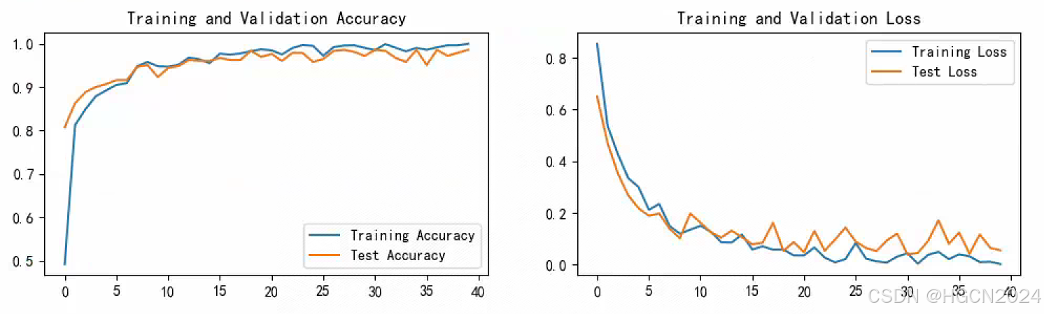
print('Done')Epoch: 1, Train_acc:49.2%, Train_loss:0.854, Test_acc:80.7%, Test_loss:0.650, Lr:1.00E-04
Epoch: 2, Train_acc:81.3%, Train_loss:0.537, Test_acc:86.3%, Test_loss:0.470, Lr:1.00E-04
Epoch: 3, Train_acc:84.9%, Train_loss:0.428, Test_acc:88.9%, Test_loss:0.353, Lr:1.00E-04
Epoch: 4, Train_acc:87.9%, Train_loss:0.334, Test_acc:90.0%, Test_loss:0.267, Lr:1.00E-04
Epoch: 5, Train_acc:89.3%, Train_loss:0.300, Test_acc:90.7%, Test_loss:0.218, Lr:1.00E-04
Epoch: 6, Train_acc:90.5%, Train_loss:0.212, Test_acc:91.6%, Test_loss:0.189, Lr:1.00E-04
Epoch: 7, Train_acc:90.9%, Train_loss:0.235, Test_acc:91.6%, Test_loss:0.197, Lr:1.00E-04
Epoch: 8, Train_acc:94.8%, Train_loss:0.149, Test_acc:94.7%, Test_loss:0.138, Lr:1.00E-04
Epoch: 9, Train_acc:95.8%, Train_loss:0.119, Test_acc:95.1%, Test_loss:0.101, Lr:1.00E-04
Epoch:10, Train_acc:94.8%, Train_loss:0.135, Test_acc:92.3%, Test_loss:0.197, Lr:1.00E-04
Epoch:11, Train_acc:94.7%, Train_loss:0.150, Test_acc:94.4%, Test_loss:0.161, Lr:1.00E-04
Epoch:12, Train_acc:95.2%, Train_loss:0.127, Test_acc:94.9%, Test_loss:0.124, Lr:1.00E-04
Epoch:13, Train_acc:96.9%, Train_loss:0.086, Test_acc:96.3%, Test_loss:0.104, Lr:1.00E-04
Epoch:14, Train_acc:96.5%, Train_loss:0.085, Test_acc:96.1%, Test_loss:0.131, Lr:1.00E-04
Epoch:15, Train_acc:95.5%, Train_loss:0.116, Test_acc:96.1%, Test_loss:0.105, Lr:1.00E-04
Epoch:16, Train_acc:97.7%, Train_loss:0.058, Test_acc:96.8%, Test_loss:0.078, Lr:1.00E-04
Epoch:17, Train_acc:97.5%, Train_loss:0.070, Test_acc:96.3%, Test_loss:0.084, Lr:1.00E-04
Epoch:18, Train_acc:97.8%, Train_loss:0.058, Test_acc:96.3%, Test_loss:0.161, Lr:1.00E-04
Epoch:19, Train_acc:98.3%, Train_loss:0.058, Test_acc:98.4%, Test_loss:0.053, Lr:1.00E-04
Epoch:20, Train_acc:98.7%, Train_loss:0.035, Test_acc:97.0%, Test_loss:0.086, Lr:1.00E-04
Epoch:21, Train_acc:98.5%, Train_loss:0.035, Test_acc:97.7%, Test_loss:0.048, Lr:1.00E-04
Epoch:22, Train_acc:97.6%, Train_loss:0.066, Test_acc:96.1%, Test_loss:0.130, Lr:1.00E-04
Epoch:23, Train_acc:99.0%, Train_loss:0.027, Test_acc:97.9%, Test_loss:0.054, Lr:1.00E-04
Epoch:24, Train_acc:99.7%, Train_loss:0.008, Test_acc:97.9%, Test_loss:0.096, Lr:1.00E-04
Epoch:25, Train_acc:99.5%, Train_loss:0.021, Test_acc:95.8%, Test_loss:0.143, Lr:1.00E-04
Epoch:26, Train_acc:97.3%, Train_loss:0.083, Test_acc:96.5%, Test_loss:0.089, Lr:1.00E-04
Epoch:27, Train_acc:99.2%, Train_loss:0.023, Test_acc:98.4%, Test_loss:0.064, Lr:1.00E-04
Epoch:28, Train_acc:99.6%, Train_loss:0.012, Test_acc:98.6%, Test_loss:0.052, Lr:1.00E-04
Epoch:29, Train_acc:99.7%, Train_loss:0.008, Test_acc:98.1%, Test_loss:0.093, Lr:1.00E-04
Epoch:30, Train_acc:99.1%, Train_loss:0.030, Test_acc:97.2%, Test_loss:0.120, Lr:1.00E-04
Epoch:31, Train_acc:98.5%, Train_loss:0.044, Test_acc:98.6%, Test_loss:0.039, Lr:1.00E-04
Epoch:32, Train_acc:99.9%, Train_loss:0.003, Test_acc:98.4%, Test_loss:0.045, Lr:1.00E-04
Epoch:33, Train_acc:99.1%, Train_loss:0.038, Test_acc:96.8%, Test_loss:0.091, Lr:1.00E-04
Epoch:34, Train_acc:98.3%, Train_loss:0.049, Test_acc:95.8%, Test_loss:0.171, Lr:1.00E-04
Epoch:35, Train_acc:99.1%, Train_loss:0.021, Test_acc:98.6%, Test_loss:0.080, Lr:1.00E-04
Epoch:36, Train_acc:98.6%, Train_loss:0.040, Test_acc:95.1%, Test_loss:0.123, Lr:1.00E-04
Epoch:37, Train_acc:99.2%, Train_loss:0.032, Test_acc:98.6%, Test_loss:0.042, Lr:1.00E-04
Epoch:38, Train_acc:99.7%, Train_loss:0.009, Test_acc:97.2%, Test_loss:0.116, Lr:1.00E-04
Epoch:39, Train_acc:99.7%, Train_loss:0.011, Test_acc:97.9%, Test_loss:0.065, Lr:1.00E-04
Epoch:40, Train_acc:100.0%, Train_loss:0.002, Test_acc:98.6%, Test_loss:0.055, Lr:1.00E-04
Done四、 结果可视化
1. Loss与Accuracy图
import matplotlib.pyplot as plt
#隐藏警告
import warnings
warnings.filterwarnings("ignore") #忽略警告信息
plt.rcParams['font.sans-serif'] = ['SimHei'] # 用来正常显示中文标签
plt.rcParams['axes.unicode_minus'] = False # 用来正常显示负号
plt.rcParams['figure.dpi'] = 100 #分辨率
epochs_range = range(epochs)
plt.figure(figsize=(12, 3))
plt.subplot(1, 2, 1)
plt.plot(epochs_range, train_acc, label='Training Accuracy')
plt.plot(epochs_range, test_acc, label='Test Accuracy')
plt.legend(loc='lower right')
plt.title('Training and Validation Accuracy')
plt.subplot(1, 2, 2)
plt.plot(epochs_range, train_loss, label='Training Loss')
plt.plot(epochs_range, test_loss, label='Test Loss')
plt.legend(loc='upper right')
plt.title('Training and Validation Loss')
plt.show()
2. 指定图片进行预测
from PIL import Image

classes = list(total_data.class_to_idx)

def predict_one_image(image_path, model, transform, classes):


    test_img = Image.open(image_path).convert('RGB')
    plt.imshow(test_img)  # 展示预测的图片

    test_img = transform(test_img)
    img = test_img.to(device).unsqueeze(0)


    model.eval()
    output = model(img)

    _,pred = torch.max(output,1)
    pred_class = classes[pred]
    print(f'预测结果是:{pred_class}')
# 预测训练集中的某张照片
predict_one_image(image_path='./PotatoPlants/Early_blight/1.JPG',
model=model,
transform=train_transforms,
classes=classes)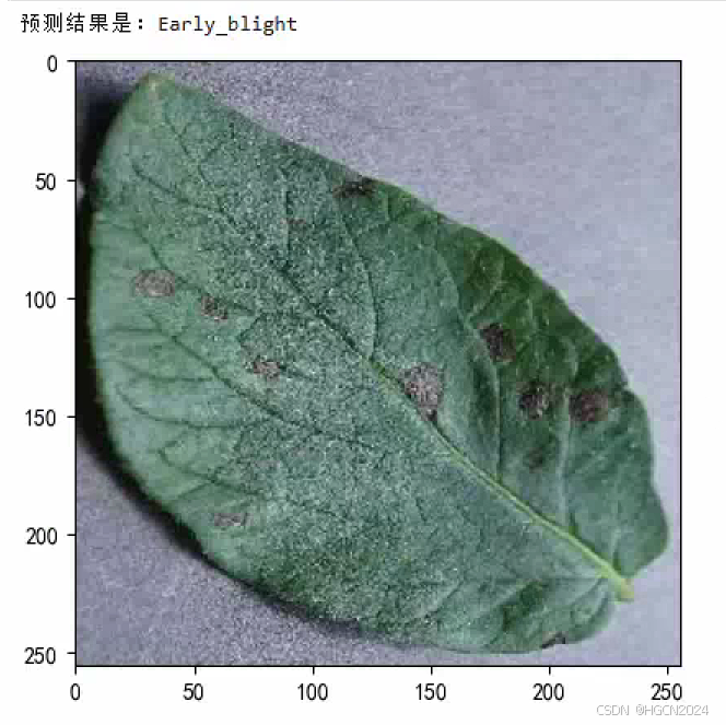
3. 模型评估
best_model.eval()
epoch_test_acc, epoch_test_loss = test(test_dl, best_model, loss_fn)

epoch_test_acc, epoch_test_loss
(0.9860788863109049, 0.0525338369313561)五、 调用官方的VGG-16网络框架
from torchvision.models import vgg16

# 加载预定义的 VGG16 模型
model = vgg16(pretrained=False)
model.classifier[6] = nn.Linear(4096, 3)  # 修改最后一层为 3 类输出
model = model.to(device)

print(f"Model loaded to: {device}")
----------------------------------------------------------------
Layer (type) Output Shape Param #
================================================================
Conv2d-1 [-1, 64, 224, 224] 1,792
ReLU-2 [-1, 64, 224, 224] 0
Conv2d-3 [-1, 64, 224, 224] 36,928
ReLU-4 [-1, 64, 224, 224] 0
MaxPool2d-5 [-1, 64, 112, 112] 0
Conv2d-6 [-1, 128, 112, 112] 73,856
ReLU-7 [-1, 128, 112, 112] 0
Conv2d-8 [-1, 128, 112, 112] 147,584
ReLU-9 [-1, 128, 112, 112] 0
MaxPool2d-10 [-1, 128, 56, 56] 0
Conv2d-11 [-1, 256, 56, 56] 295,168
ReLU-12 [-1, 256, 56, 56] 0
Conv2d-13 [-1, 256, 56, 56] 590,080
ReLU-14 [-1, 256, 56, 56] 0
Conv2d-15 [-1, 256, 56, 56] 590,080
ReLU-16 [-1, 256, 56, 56] 0
MaxPool2d-17 [-1, 256, 28, 28] 0
Conv2d-18 [-1, 512, 28, 28] 1,180,160
ReLU-19 [-1, 512, 28, 28] 0
Conv2d-20 [-1, 512, 28, 28] 2,359,808
ReLU-21 [-1, 512, 28, 28] 0
Conv2d-22 [-1, 512, 28, 28] 2,359,808
ReLU-23 [-1, 512, 28, 28] 0
MaxPool2d-24 [-1, 512, 14, 14] 0
Conv2d-25 [-1, 512, 14, 14] 2,359,808
ReLU-26 [-1, 512, 14, 14] 0
Conv2d-27 [-1, 512, 14, 14] 2,359,808
ReLU-28 [-1, 512, 14, 14] 0
Conv2d-29 [-1, 512, 14, 14] 2,359,808
ReLU-30 [-1, 512, 14, 14] 0
MaxPool2d-31 [-1, 512, 7, 7] 0
AdaptiveAvgPool2d-32 [-1, 512, 7, 7] 0
Linear-33 [-1, 4096] 102,764,544
ReLU-34 [-1, 4096] 0
Dropout-35 [-1, 4096] 0
Linear-36 [-1, 4096] 16,781,312
ReLU-37 [-1, 4096] 0
Dropout-38 [-1, 4096] 0
Linear-39 [-1, 3] 12,291
================================================================
Total params: 134,272,835
Trainable params: 134,272,835
Non-trainable params: 0
----------------------------------------------------------------
Input size (MB): 0.57
Forward/backward pass size (MB): 218.77
Params size (MB): 512.21
Estimated Total Size (MB): 731.56
----------------------------------------------------------------可见和自己搭建的VGG16模型基本一致
六、在不影响准确率的前提下轻量化模型
from torchvision.models import vgg16
import torch.nn as nn

# 加载预定义的 VGG16 模型
model = vgg16(pretrained=False)

# 替换全连接层
model.classifier = nn.Sequential(
    nn.Linear(512 * 7 * 7, 1024),  # 从 4096 缩减到 1024
    nn.ReLU(),
    nn.Dropout(0.5),
    nn.Linear(1024, 256),  # 第二层从 4096 缩减到 256
    nn.ReLU(),
    nn.Dropout(0.5),
    nn.Linear(256, 3)  # 输出层保持不变
)

model = model.to(device)
将全连接层分别缩减到1024和256,输出不变
----------------------------------------------------------------
        Layer (type)               Output Shape         Param #
================================================================
            Conv2d-1         [-1, 64, 224, 224]           1,792
              ReLU-2         [-1, 64, 224, 224]               0
            Conv2d-3         [-1, 64, 224, 224]          36,928
              ReLU-4         [-1, 64, 224, 224]               0
         MaxPool2d-5         [-1, 64, 112, 112]               0
            Conv2d-6        [-1, 128, 112, 112]          73,856
              ReLU-7        [-1, 128, 112, 112]               0
            Conv2d-8        [-1, 128, 112, 112]         147,584
              ReLU-9        [-1, 128, 112, 112]               0
        MaxPool2d-10          [-1, 128, 56, 56]               0
           Conv2d-11          [-1, 256, 56, 56]         295,168
             ReLU-12          [-1, 256, 56, 56]               0
           Conv2d-13          [-1, 256, 56, 56]         590,080
             ReLU-14          [-1, 256, 56, 56]               0
           Conv2d-15          [-1, 256, 56, 56]         590,080
             ReLU-16          [-1, 256, 56, 56]               0
        MaxPool2d-17          [-1, 256, 28, 28]               0
           Conv2d-18          [-1, 512, 28, 28]       1,180,160
             ReLU-19          [-1, 512, 28, 28]               0
           Conv2d-20          [-1, 512, 28, 28]       2,359,808
             ReLU-21          [-1, 512, 28, 28]               0
           Conv2d-22          [-1, 512, 28, 28]       2,359,808
             ReLU-23          [-1, 512, 28, 28]               0
        MaxPool2d-24          [-1, 512, 14, 14]               0
           Conv2d-25          [-1, 512, 14, 14]       2,359,808
             ReLU-26          [-1, 512, 14, 14]               0
           Conv2d-27          [-1, 512, 14, 14]       2,359,808
             ReLU-28          [-1, 512, 14, 14]               0
           Conv2d-29          [-1, 512, 14, 14]       2,359,808
             ReLU-30          [-1, 512, 14, 14]               0
        MaxPool2d-31            [-1, 512, 7, 7]               0
AdaptiveAvgPool2d-32            [-1, 512, 7, 7]               0
           Linear-33                 [-1, 1024]      25,691,136
             ReLU-34                 [-1, 1024]               0
          Dropout-35                 [-1, 1024]               0
           Linear-36                  [-1, 256]         262,400
             ReLU-37                  [-1, 256]               0
          Dropout-38                  [-1, 256]               0
           Linear-39                    [-1, 3]             771
================================================================
Total params: 40,668,995
Trainable params: 40,668,995
Non-trainable params: 0
----------------------------------------------------------------
Input size (MB): 0.57
Forward/backward pass size (MB): 218.62
Params size (MB): 155.14
Estimated Total Size (MB): 374.33
----------------------------------------------------------------
可以看到参数量缩小为原来的约1/3
Epoch: 1, Train_acc:53.6%, Train_loss:0.924, Test_acc:79.6%, Test_loss:0.712, Lr:5.00E-04
Epoch: 2, Train_acc:74.7%, Train_loss:0.664, Test_acc:82.6%, Test_loss:0.487, Lr:5.00E-04
Epoch: 3, Train_acc:81.6%, Train_loss:0.515, Test_acc:81.9%, Test_loss:0.477, Lr:5.00E-04
Epoch: 4, Train_acc:82.3%, Train_loss:0.499, Test_acc:84.5%, Test_loss:0.436, Lr:5.00E-04
Epoch: 5, Train_acc:83.6%, Train_loss:0.463, Test_acc:83.1%, Test_loss:0.480, Lr:5.00E-04
Epoch: 6, Train_acc:83.7%, Train_loss:0.464, Test_acc:85.2%, Test_loss:0.428, Lr:5.00E-04
Epoch: 7, Train_acc:86.1%, Train_loss:0.411, Test_acc:86.5%, Test_loss:0.388, Lr:5.00E-04
Epoch: 8, Train_acc:85.2%, Train_loss:0.435, Test_acc:86.1%, Test_loss:0.367, Lr:5.00E-04
Epoch: 9, Train_acc:85.9%, Train_loss:0.404, Test_acc:88.2%, Test_loss:0.334, Lr:5.00E-04
Epoch:10, Train_acc:84.4%, Train_loss:0.446, Test_acc:84.9%, Test_loss:0.392, Lr:5.00E-04
Epoch:11, Train_acc:85.6%, Train_loss:0.400, Test_acc:87.9%, Test_loss:0.376, Lr:5.00E-04
Epoch:12, Train_acc:85.5%, Train_loss:0.372, Test_acc:84.7%, Test_loss:0.417, Lr:5.00E-04
Epoch:13, Train_acc:86.1%, Train_loss:0.402, Test_acc:89.1%, Test_loss:0.268, Lr:5.00E-04
Epoch:14, Train_acc:89.1%, Train_loss:0.307, Test_acc:88.4%, Test_loss:0.321, Lr:5.00E-04
Epoch:15, Train_acc:89.7%, Train_loss:0.291, Test_acc:87.5%, Test_loss:0.326, Lr:5.00E-04
Epoch:16, Train_acc:88.3%, Train_loss:0.312, Test_acc:89.3%, Test_loss:0.310, Lr:5.00E-04
Epoch:17, Train_acc:88.1%, Train_loss:0.338, Test_acc:90.5%, Test_loss:0.239, Lr:5.00E-04
Epoch:18, Train_acc:89.2%, Train_loss:0.279, Test_acc:91.0%, Test_loss:0.242, Lr:5.00E-04
Epoch:19, Train_acc:90.8%, Train_loss:0.259, Test_acc:87.2%, Test_loss:0.338, Lr:5.00E-04
Epoch:20, Train_acc:90.7%, Train_loss:0.248, Test_acc:88.4%, Test_loss:0.372, Lr:5.00E-04
Epoch:21, Train_acc:87.6%, Train_loss:0.338, Test_acc:90.7%, Test_loss:0.251, Lr:5.00E-04
Epoch:22, Train_acc:89.9%, Train_loss:0.260, Test_acc:89.3%, Test_loss:0.283, Lr:5.00E-04
Epoch:23, Train_acc:91.4%, Train_loss:0.235, Test_acc:87.0%, Test_loss:0.368, Lr:5.00E-04
Epoch:24, Train_acc:93.1%, Train_loss:0.197, Test_acc:91.4%, Test_loss:0.210, Lr:5.00E-04
Epoch:25, Train_acc:92.7%, Train_loss:0.178, Test_acc:91.9%, Test_loss:0.220, Lr:5.00E-04
Epoch:26, Train_acc:93.5%, Train_loss:0.200, Test_acc:95.6%, Test_loss:0.149, Lr:5.00E-04
Epoch:27, Train_acc:93.8%, Train_loss:0.181, Test_acc:92.1%, Test_loss:0.208, Lr:5.00E-04
Epoch:28, Train_acc:94.4%, Train_loss:0.173, Test_acc:93.7%, Test_loss:0.220, Lr:5.00E-04
Epoch:29, Train_acc:94.8%, Train_loss:0.149, Test_acc:95.4%, Test_loss:0.127, Lr:5.00E-04
Epoch:30, Train_acc:95.1%, Train_loss:0.153, Test_acc:94.2%, Test_loss:0.143, Lr:5.00E-04
Epoch:31, Train_acc:95.0%, Train_loss:0.136, Test_acc:94.9%, Test_loss:0.143, Lr:5.00E-04
Epoch:32, Train_acc:93.9%, Train_loss:0.169, Test_acc:94.7%, Test_loss:0.149, Lr:5.00E-04
Epoch:33, Train_acc:94.6%, Train_loss:0.138, Test_acc:93.5%, Test_loss:0.202, Lr:5.00E-04
Epoch:34, Train_acc:96.0%, Train_loss:0.126, Test_acc:96.5%, Test_loss:0.088, Lr:5.00E-04
Epoch:35, Train_acc:96.7%, Train_loss:0.102, Test_acc:97.0%, Test_loss:0.095, Lr:5.00E-04
Epoch:36, Train_acc:94.9%, Train_loss:0.142, Test_acc:93.5%, Test_loss:0.169, Lr:5.00E-04
Epoch:37, Train_acc:95.8%, Train_loss:0.124, Test_acc:93.3%, Test_loss:0.171, Lr:5.00E-04
Epoch:38, Train_acc:95.5%, Train_loss:0.122, Test_acc:95.6%, Test_loss:0.120, Lr:5.00E-04
Epoch:39, Train_acc:94.9%, Train_loss:0.144, Test_acc:97.4%, Test_loss:0.071, Lr:5.00E-04
Epoch:40, Train_acc:96.4%, Train_loss:0.104, Test_acc:96.3%, Test_loss:0.079, Lr:5.00E-04
Done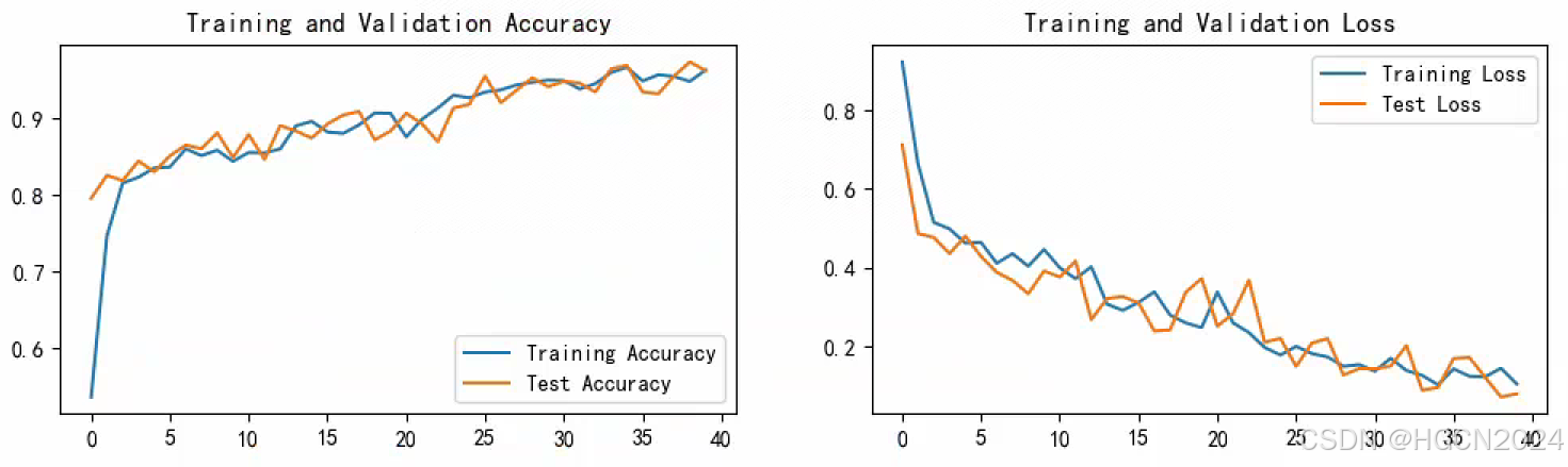
对预测准确率基本没有影响
七、学习小结
通过自己搭建VGG-16网络,使我加深了对卷积神经网络的理解。VGG-16的网络构造并不复杂,只要按照合理的层叠规则,结合激活函数、池化操作等,就能有效提取图像的特征。
模型轻量化的探索是本次学习的重点,通过减少全连接层的规模,可以在不影响模型性能的前提下,显著减少参数量和计算量。模型计算量减少的同时,分类准确率几乎没有下降。


 被折叠的 条评论
为什么被折叠?
被折叠的 条评论
为什么被折叠?
 到【灌水乐园】发言


