1-逻辑回归实战

最新推荐文章于 2024-01-07 18:02:57 发布

进击的小杨人

最新推荐文章于 2024-01-07 18:02:57 发布

阅读量324

点赞数

分类专栏：机器学习实战文章标签：机器学习逻辑回归 python

本文链接：https://blog.csdn.net/weixin_42600072/article/details/88432110

版权

机器学习实战专栏收录该内容

23 篇文章 7 订阅

订阅专栏

Logistic Regression

The data

我们将建立一个逻辑回归模型来预测一个学生是否被大学录取。假设你是一个大学系的管理员，你想根据两次考试的结果来决定每个申请人的录取机会。你有以前的申请人的历史数据，你可以用它作为逻辑回归的训练集。对于每一个培训例子，你有两个考试的申请人的分数和录取决定。为了做到这一点，我们将建立一个分类模型，根据考试成绩估计入学概率。

import numpy as np
import pandas as pd
import matplotlib.pyplot as plt

import os
path = 'data' + os.sep + 'LogiReg_data.txt'
pdData = pd.read_csv(path, header=None, names=['Exam1','Exam2','Admitted'])
pdData.head()

	Exam1	Exam2	Admitted
0	34.623660	78.024693	0
1	30.286711	43.894998	0
2	35.847409	72.902198	0
3	60.182599	86.308552	1
4	79.032736	75.344376	1

pdData.shape

(100, 3)

positive = pdData[pdData['Admitted'] == 1]
negative = pdData[pdData['Admitted'] == 0]
fig,ax = plt.subplots(figsize=(10,5))
ax.scatter(positive['Exam1'], positive['Exam2'], s=30, c='b',marker='o', label='Admitted')
ax.scatter(negative['Exam1'], negative['Exam2'], s=30, c='r',marker='x', label='Not admitted')
plt.legend()
ax.set_xlabel('Exam1')
ax.set_ylabel('Exam2')
plt.show()

在这里插入图片描述

The logistic regression

目标：建立分类器（求解出三个参数 $\theta_0 \theta_1 \theta_2 $）

设定阈值，根据阈值判断录取结果

要完成的模块

sigmoid : 映射到概率的函数
model : 返回预测结果值
cost : 根据参数计算损失
gradient : 计算每个参数的梯度方向
descent : 进行参数更新
accuracy: 计算精度

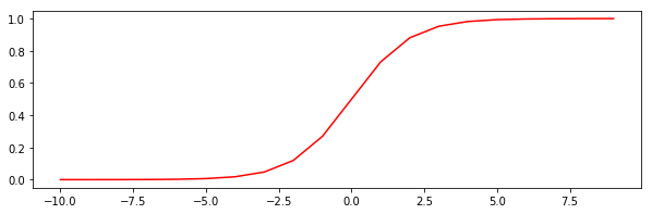
sigmoid函数

$\frac{1}{1+e^{-z}}$

def sigmoid(z):
    return 1 / (1 + np.exp(-z))

nums = np.arange(-10,10,step=1)
fig,ax = plt.subplots(figsize=(10,3))
ax.plot(nums,sigmoid(nums),'r')

[<matplotlib.lines.Line2D at 0x8b79518>]

在这里插入图片描述

model

$\begin{array}{ccc} \begin{pmatrix}\theta_{0} & \theta_{1} & \theta_{2}\end{pmatrix} & \times & \begin{pmatrix}1\\ x_{1}\\ x_{2} \end{pmatrix}\end{array}=\theta_{0}+\theta_{1}x_{1}+\theta_{2}x_{2}$

def model(X, theta):
    return sigmoid(np.dot(X, theta.T))

pdData.insert(0,'Ones',1)

pd.as_matrix()将frame转换为其Numpy数组表示

print(pdData.head())
orig_data = pdData.as_matrix()
cols = orig_data.shape[1]
X = orig_data[:,0:cols-1]
y = orig_data[:,cols-1:cols]
theta = np.zeros([1,3])

   Ones      Exam1      Exam2  Admitted
0     1  34.623660  78.024693         0
1     1  30.286711  43.894998         0
2     1  35.847409  72.902198         0
3     1  60.182599  86.308552         1
4     1  79.032736  75.344376         1


C:\ProgramData\Anaconda3\lib\site-packages\ipykernel_launcher.py:2: FutureWarning: Method .as_matrix will be removed in a future version. Use .values instead.

X[:5]

array([[ 1.        , 34.62365962, 78.02469282],
       [ 1.        , 30.28671077, 43.89499752],
       [ 1.        , 35.84740877, 72.90219803],
       [ 1.        , 60.18259939, 86.3085521 ],
       [ 1.        , 79.03273605, 75.34437644]])

y[:5]

array([[0.],
       [0.],
       [0.],
       [1.],
       [1.]])

theta

array([[0., 0., 0.]])

print(X.shape,y.shape,theta.shape)

(100, 3) (100, 1) (1, 3)

损失函数

$D(h_\theta(x), y) = -y\log(h_\theta(x)) - (1-y)\log(1-h_\theta(x))$
求平均损失
$J(\theta)=\frac{1}{n}\sum_{i=1}^{n} D(h_\theta(x_i), y_i)$

def cost(X,y,theta):
    left = np.multiply(-y, np.log(model(X,theta)))
    right = np.multiply(1 - y, np.log(1 - model(X,theta)))
    return np.sum(left - right) / len(X)

cost(X,y,theta)

0.6931471805599453

计算梯度

$\frac{\partial J}{\partial \theta_j}=-\frac{1}{m}\sum_{i=1}^n (y_i - h_\theta (x_i))x_{ij}$

def gradient(X,y,theta):
    grad = np.zeros(theta.shape)
    error = model(X, theta) - y
    for j in range(len(theta.ravel())):
        term = np.multiply(error, X)
        grad[0,j] = np.sum(term) / len(X)
    return grad

gradient(X,y,theta)

array([[-23.37205879, -23.37205879, -23.37205879]])

Gradient descent

比较3中不同梯度下降方法

STOP_ITER = 0
STOP_COST = 1
STOP_GRAD = 2
def stopCriterion(type, value, threshold):
    #设定三种不同的停止策略
    if type == STOP_ITER:
        return value > threshold
    elif type == STOP_COST:
        return abs(value[-1]-value[-2]) < threshold
    else:
        return np.linalg.norm(value) < threshold

import numpy.random
#洗牌
def shuffleData(data):
    np.random.shuffle(data)
    cols = data.shape[1]
    X = data[:,0:cols-1]
    y = data[:,cols-1:cols]
    return X,y

import time
def  descent(data,theta, batchSize,stopType,thresh,alpha):
    init_time = time.time()
    i = 0 #迭代次数
    k = 0 #bacth大小
    X,y = shuffleData(data)
    grad = np.zeros(theta.shape) #梯度
    costs = [cost(X,y,theta)]  #损失值
    
    while True:
        grad = gradient(X[k:k+batchSize],y[k:k+batchSize],theta)
        k += batchSize #取batch个数据
        if k >= n:
            k = 0
            X,y = shuffleData(data)
        theta = theta - alpha * grad #参数更新
        costs.append(cost(X,y,theta)) #计算新的损失
        i += 1
        
        if stopType == STOP_ITER:
            value = i
        elif stopType == STOP_COST:
            value = costs
        elif stopType == STOP_GRAD:
            value = grad
        if stopCriterion(stopType, value, thresh):
            break
    return theta, i-1, costs, grad, time.time()-init_time

def runExpe(data, theta, batchSize, stopType, thresh, alpha):
    #import pdb; pdb.set_trace();
    theta, iter, costs, grad, dur = descent(data, theta, batchSize, stopType, thresh, alpha)
    name = "Original" if (data[:,1]>2).sum() > 1 else "Scaled"
    name += " data - learning rate: {} - ".format(alpha)
    if batchSize==n: strDescType = "Gradient"
    elif batchSize==1:  strDescType = "Stochastic"
    else: strDescType = "Mini-batch ({})".format(batchSize)
    name += strDescType + " descent - Stop: "
    if stopType == STOP_ITER: strStop = "{} iterations".format(thresh)
    elif stopType == STOP_COST: strStop = "costs change < {}".format(thresh)
    else: strStop = "gradient norm < {}".format(thresh)
    name += strStop
    print ("***{}\nTheta: {} - Iter: {} - Last cost: {:03.2f} - Duration: {:03.2f}s".format(
        name, theta, iter, costs[-1], dur))
    fig, ax = plt.subplots(figsize=(12,4))
    ax.plot(np.arange(len(costs)), costs, 'r')
    ax.set_xlabel('Iterations')
    ax.set_ylabel('Cost')
    ax.set_title(name.upper() + ' - Error vs. Iteration')
    return theta

不同的停止策略

设定迭代次数

#选择的梯度下降方法是基于所有样本的
n=100
runExpe(orig_data, theta, n, STOP_ITER, thresh=5000, alpha=0.000001)

***Original data - learning rate: 1e-06 - Gradient descent - Stop: 5000 iterations
Theta: [[0.00534501 0.00534501 0.00534501]] - Iter: 5000 - Last cost: 0.63 - Duration: 1.48s





array([[0.00534501, 0.00534501, 0.00534501]])

在这里插入图片描述

根据损失值停止
设定阈值 1E-6, 差不多需要110 000次迭代

runExpe(orig_data, theta, n, STOP_COST, thresh=0.001, alpha=0.001)

***Original data - learning rate: 0.001 - Gradient descent - Stop: costs change < 0.001
Theta: [[0.00603476 0.00603476 0.00603476]] - Iter: 66 - Last cost: 0.63 - Duration: 0.04s





array([[0.00603476, 0.00603476, 0.00603476]])

png

根据梯度变化停止
设定阈值 0.05,差不多需要40 000次迭代

runExpe(orig_data, theta, n, STOP_GRAD, thresh=0.05, alpha=0.001)

---------------------------------------------------------------------------

KeyboardInterrupt                         Traceback (most recent call last)

<ipython-input-26-885c52625e09> in <module>
----> 1 runExpe(orig_data, theta, n, STOP_GRAD, thresh=0.05, alpha=0.001)


<ipython-input-21-c025af6684d1> in runExpe(data, theta, batchSize, stopType, thresh, alpha)
      1 def runExpe(data, theta, batchSize, stopType, thresh, alpha):
      2     #import pdb; pdb.set_trace();
----> 3     theta, iter, costs, grad, dur = descent(data, theta, batchSize, stopType, thresh, alpha)
      4     name = "Original" if (data[:,1]>2).sum() > 1 else "Scaled"
      5     name += " data - learning rate: {} - ".format(alpha)


<ipython-input-20-2bf97e800a62> in descent(data, theta, batchSize, stopType, thresh, alpha)
     15             X,y = shuffleData(data)
     16         theta = theta - alpha * grad #参数更新
---> 17         costs.append(cost(X,y,theta)) #计算新的损失
     18         i += 1
     19 


<ipython-input-14-50079328a47e> in cost(X, y, theta)
      1 def cost(X,y,theta):
      2     left = np.multiply(-y, np.log(model(X,theta)))
----> 3     right = np.multiply(1 - y, np.log(1 - model(X,theta)))
      4     return np.sum(left - right) / len(X)


<ipython-input-7-068d3efff1d9> in model(X, theta)
      1 def model(X, theta):
----> 2     return sigmoid(np.dot(X, theta.T))


KeyboardInterrupt:

我们来尝试下对数据进行标准化将数据按其属性(按列进行)减去其均值，然后除以其方差。最后得到的结果是，对每个属性/每列来说所有数据都聚集在0附近，方差值为1

from sklearn import preprocessing as pp

scaled_data = orig_data.copy()
scaled_data[:, 1:3] = pp.scale(orig_data[:, 1:3])

runExpe(scaled_data, theta, n, STOP_ITER, thresh=5000, alpha=0.001)

runExpe(scaled_data, theta, n, STOP_GRAD, thresh=0.02, alpha=0.001)

theta = runExpe(scaled_data, theta, 1, STOP_GRAD, thresh=0.002/5, alpha=0.001)

精度

#设定阈值
def predict(X, theta):
    for x in model(X, theta):
        if x > 0.5: return 1
        else: return 0

scaled_X = scaled_data[:, :3]
y = scaled_data[:, 3]
predictions = predict(scaled_X, theta)
correct = [1 if ((a == 1 and b == 1) or (a == 0 and b == 0)) else 0 for (a, b) in zip(predictions, y)]
accuracy = (sum(map(int, correct)) % len(correct))
print ('accuracy = {0}%'.format(accuracy))

---------------------------------------------------------------------------

NameError                                 Traceback (most recent call last)

<ipython-input-28-96295c8a28b2> in <module>
----> 1 scaled_X = scaled_data[:, :3]
      2 y = scaled_data[:, 3]
      3 predictions = predict(scaled_X, theta)
      4 correct = [1 if ((a == 1 and b == 1) or (a == 0 and b == 0)) else 0 for (a, b) in zip(predictions, y)]
      5 accuracy = (sum(map(int, correct)) % len(correct))


NameError: name 'scaled_data' is not defined

进击的小杨人

关注

0
点赞
踩
0

收藏

觉得还不错? 一键收藏
1
评论
1-逻辑回归实战

Logistic RegressionThe data我们将建立一个逻辑回归模型来预测一个学生是否被大学录取。假设你是一个大学系的管理员，你想根据两次考试的结果来决定每个申请人的录取机会。你有以前的申请人的历史数据，你可以用它作为逻辑回归的训练集。对于每一个培训例子，你有两个考试的申请人的分数和录取决定。为了做到这一点，我们将建立一个分类模型，根据考试成绩估计入学概率。import nump...
复制链接

扫一扫