根据颜色不同进行匹配

一、色彩阀值化处理——利用openCV-python中inRange()等相关函数

# -*- coding: utf-8 -*-
import numpy as np
import collections
import cv2
import numpy as np
filename = 'E:/lixueqian/openCV/00637aaa.jpg'
# 定义字典存放颜色分量上下限
# 例如：{颜色: [min分量, max分量]}
# {'red': [array([160,  43,  46]), array([179, 255, 255])]}
def getColorList():
    dict = collections.defaultdict(list)

    # 黑色
    lower_black = np.array([0, 0, 0])
    upper_black = np.array([180, 255, 46])
    color_list = []
    color_list.append(lower_black)
    color_list.append(upper_black)
    dict['black'] = color_list

    # #灰色
    # lower_gray = np.array([0, 0, 46])
    # upper_gray = np.array([180, 43, 220])
    # color_list = []
    # color_list.append(lower_gray)
    # color_list.append(upper_gray)
    # dict['gray']=color_list

    # 白色
    lower_white = np.array([0, 0, 221])
    upper_white = np.array([180, 30, 255])
    color_list = []
    color_list.append(lower_white)
    color_list.append(upper_white)
    dict['white'] = color_list

    # 红色
    lower_red = np.array([156, 43, 46])
    upper_red = np.array([180, 255, 255])
    color_list = []
    color_list.append(lower_red)
    color_list.append(upper_red)
    dict['red'] = color_list

    # 红色2
    lower_red = np.array([0, 43, 46])
    upper_red = np.array([10, 255, 255])
    color_list = []
    color_list.append(lower_red)
    color_list.append(upper_red)
    dict['red2'] = color_list

    # 橙色
    lower_orange = np.array([11, 43, 46])
    upper_orange = np.array([25, 255, 255])
    color_list = []
    color_list.append(lower_orange)
    color_list.append(upper_orange)
    dict['orange'] = color_list

    # 黄色
    lower_yellow = np.array([26, 43, 46])
    upper_yellow = np.array([34, 255, 255])
    color_list = []
    color_list.append(lower_yellow)
    color_list.append(upper_yellow)
    dict['yellow'] = color_list

    # 绿色
    lower_green = np.array([35, 43, 46])
    upper_green = np.array([77, 255, 255])
    color_list = []
    color_list.append(lower_green)
    color_list.append(upper_green)
    dict['green'] = color_list

    # 青色
    lower_cyan = np.array([78, 43, 46])
    upper_cyan = np.array([99, 255, 255])
    color_list = []
    color_list.append(lower_cyan)
    color_list.append(upper_cyan)
    dict['cyan'] = color_list

    # 蓝色
    lower_blue = np.array([100, 43, 46])
    upper_blue = np.array([124, 255, 255])
    color_list = []
    color_list.append(lower_blue)
    color_list.append(upper_blue)
    dict['blue'] = color_list

    # 紫色
    lower_purple = np.array([125, 43, 46])
    upper_purple = np.array([155, 255, 255])
    color_list = []
    color_list.append(lower_purple)
    color_list.append(upper_purple)
    dict['purple'] = color_list

    return dict
# 处理图片
def get_color(frame):
    #print('go in get_color')
    hsv = cv2.cvtColor(frame, cv2.COLOR_BGR2HSV)
    maxsum = -100
    color = None
    color_dict = getColorList()
    for d in color_dict:
        mask = cv2.inRange(hsv, color_dict[d][0], color_dict[d][1])
        cv2.imwrite(d + '.jpg', mask)
        binary = cv2.threshold(mask, 127, 255, cv2.THRESH_BINARY)[1]
        binary = cv2.dilate(binary, None, iterations=2)
        img, cnts, hiera = cv2.findContours(binary.copy(), cv2.RETR_EXTERNAL, cv2.CHAIN_APPROX_SIMPLE)
        sum = 0
        for c in cnts:
            sum += cv2.contourArea(c)
        if sum > maxsum:
            maxsum = sum
            color = d

    return color


if __name__ == '__main__':
    frame = cv2.imread(filename)
    a=get_color(frame)
    print(a)

二、图像颜色直方图的提取与匹配（主要思路：提取特征+计算距离）

1. 图像颜色直方图的提取

   假设一幅图像G的颜色（或灰度）由N级组成，每一级颜色值用q(i),(i=1,2,3…N)表示。在整幅图像中，具有q(i)颜色值的像素数为hi,则各级颜色值像素统计值为h1,h2,…hN，构成了图像的特征值——颜色直方图。
   颜色直方图特征提取是统计图像中每种颜色像素的数目。将颜色空间等距离分组取值，然后再统计每组中对应的像素数目，从而得到整个图像的颜色直方图。
   函数: cv2.calcHist([images],[ channels], mask,[histSize],[ranges], hist, accumulate ) #返回hist
   第二个参数是用于计算直方图的通道
   第三个参数是Mask，没有使用就用None
   第四个参数是histSize，表示这个直方图分成多少份（即多少个直方柱）
   第五个参数是表示直方图中各个像素的值，[0.0, 256.0]表示直方图能表示像素值从0.0到256的像素。

def solve_hist(img):
    # 计算图片的颜色分布直方图，返回3*n*1的列表，3代表3个颜色，n为16，代表颜色分段的个数
   # color_num = img.shape[0] * img.shape[1]
    hist_list = []
    for i in [0, 1, 2]:
        hist = cv2.calcHist([img], [i], None, [16], [0, 255])  # 彩色图有三个通道，通道b:0,g:1,r:2
        #hist是属于每个颜色区间里像素的个数
        #hist = hist / color_num #* 100
        hist_list.append(hist)
    return hist_list

2. 匹配
   （1）欧式距离
   假设查询实例图像的直方图用G（g1,g2,…gN）表示，数据库中的目标图像的直方图用S（s1,s2,…sN）表示，可以将这两个直方图看作欧式空间的两个点，利用欧氏距离来描述他们的相似性。 欧式距离的值越接近零，则表示两幅图像越相似。

def solve_hist_distance(img1, img2):
    hist_list1 = solve_hist(img1)
    hist_list2 = solve_hist(img2)
    b_distance, g_distance, r_distance = 0, 0, 0
    img1_b_hist, img1_g_hist, img1_r_hist = hist_list1
    img2_b_hist, img2_g_hist, img2_r_hist = hist_list2
    for i in range(len(img1_b_hist)):
        b_distance += (img1_b_hist[i] - img2_b_hist[i]) ** 2
    for i in range(len(img1_g_hist)):
        g_distance += (img1_g_hist[i] - img2_g_hist[i]) ** 2
    for i in range(len(img1_r_hist)):
        r_distance += (img1_r_hist[i] - img2_r_hist[i]) ** 2
    print (b_distance, g_distance, r_distance)
    return b_distance, g_distance, r_distance

  本段代码执行结果返回三个结果，不利于找到阈值，不做深入研究。

（2）余弦距离（相似度）
严格来讲余弦距离不是距离，而只是相似性。其他距离直接测量两个高维空间上的点的距离，如果距离为0则两个点“相同”；余弦的结果为在[0，1]之中，如果为 1，只能确定两者完全相关、完全相似。假设两用户同时对两件商品评分，向量分别为(3,3)和(5,5)，这两位用户对两件商品的喜好其实是一样的。例如，当两条新闻向量夹角余弦等于1时，这两条新闻完全重复（用这个办法可以删除爬虫所收集网页中的重复网页）；当夹角的余弦值接近于1时，两条新闻相似（可以用作文本分类）；夹角的余弦越小，两条新闻越不相关。
优点：余弦距离根据向量方向来判断向量相似度，与向量各个维度的相对大小有关，不受各个维度直接数值影响。
（代码在后边）

（3）欧式距离与余弦距离的对比
余弦距离使用两个向量夹角的余弦值作为衡量两个个体间差异的大小。相比欧氏距离，余弦距离更加注重两个向量在方向上的差异。

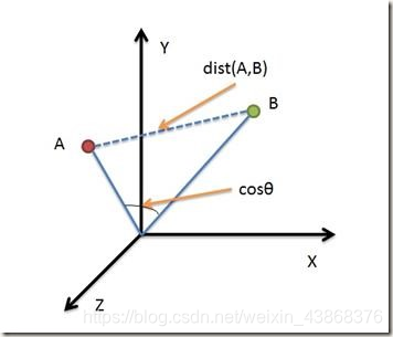
从上图可以看出，欧氏距离衡量的是空间各点的绝对距离，跟各个点所在的位置坐标直接相关；而余弦距离衡量的是空间向量的夹角，更加体现在方向上的差异，而不是位置。如果保持A点位置不变，B点朝原方向远离坐标轴原点，那么这个时候余弦距离是保持不变的（因为夹角没有发生变化），而A、B两点的距离显然在发生改变，这就是欧氏距离和余弦距离之间的不同之处。
欧氏距离和余弦距离各自有不同的计算方式和衡量特征，因此它们适用于不同的数据分析模型：
1）欧氏距离能够体现个体数值特征的绝对差异，所以更多的用于需要从维度的数值大小中体现差异的分析，如使用用户行为指标分析用户价值的相似度或差异。
2）余弦距离更多的是从方向上区分差异，而对绝对的数值不敏感，更多的用于使用用户对内容评分来区分兴趣的相似度和差异，同时修正了用户间可能存在的度量标准不统一的问题（因为余弦距离对绝对数值不敏感）。
函数distance.cosine是计算一维数组之间的余弦距离（余弦距离是1-cos<u,v>）
代码：

def solve_hist_distance_cos(img1, img2):
    hist_list1 = solve_hist(img1)
    hist_list2 = solve_hist(img2)
    b_distance, g_distance, r_distance = 0, 0, 0
    img1_b_hist, img1_g_hist, img1_r_hist = hist_list1
    img2_b_hist, img2_g_hist, img2_r_hist = hist_list2
    b_distance = 1-distance.cosine(img1_b_hist, img2_b_hist)
    g_distance = 1-distance.cosine(img1_g_hist, img2_g_hist)
    r_distance = 1-distance.cosine(img1_r_hist, img2_r_hist)
    return (b_distance + g_distance + r_distance) / 3

用余弦距离运行的结果爽歪歪：
0.416310465274 不相似
0.833218993694 相似
0.7659640513 相似
0.843376579073 相似
0.0377763099575 不相似

本来不知道有这个可以直接计算余弦距离的函数，从网上找了一点公式需要自己修改，感觉还是很锻炼能力的，现在就来操作一波！
自己编写的计算余弦相似度的函数：

def solve_hist_distance_cos1(img1, img2):
    hist_list1 = solve_hist(img1)
    hist_list2 = solve_hist(img2)
    img1_b_hist, img1_g_hist, img1_r_hist = hist_list1
    img2_b_hist, img2_g_hist, img2_r_hist = hist_list2
    si=len(img1_b_hist)
    #s = sum(img1_b_hist[item] * img2_b_hist[item] for item in si])
    #s =[a * b for a, b in zip(img1_b_hist,img2_b_hist)]#list len=16 对应元素相乘
    s=np.dot(img1_b_hist.T,img2_b_hist) #点乘
    den1 = math.sqrt(sum([pow(img1_b_hist[item], 2) for item in range(0,si)]))#不能直接用int进行迭代，而必须加个range。
    den2 = math.sqrt(sum([pow(img2_b_hist[item], 2) for item in range(0,si)]))
    b_distance=s / (den1 * den2)
    return   b_distance

三、通过降维提取图像颜色直方图并匹配

#做一个rgb的直方图
import cv2
import numpy as np
import math
def create_rgb_hist(img):
    h, w, c = img.shape
    rgbHist = np.zeros([16*16*16,1],np.float32) # blue 16个 green 16个 red16个
    bsize = 256/16 # 直方图有256个bins 除以16 =16 
    for row in range(h):
        for col in range(w):
            b = img[row, col, 0]
            g = img[row, col, 1]
            r = img[row, col, 2]
            index = np.int(b/bsize)*16*16 + np.int(g/bsize)*16 + np.int(r/bsize) #降维操作 把256*256*256 转成16*16*16
            rgbHist[np.int(index), 0] +=1
    return rgbHist
#之后再进行RGB直方图的比较
def hist_compare(img1,img2):
    hist1 = create_rgb_hist(img1)
    hist2 = create_rgb_hist(img2)
    match1 = cv2.compareHist(hist1, hist2, cv2.HISTCMP_BHATTACHARYYA) # 巴氏距离 越小图片的相似度越高
    match2 = cv2.compareHist(hist1, hist2, cv2.HISTCMP_CORREL) # 相关性 越大图片的相似度越高
    match3 = cv2.compareHist(hist1, hist2, cv2.HISTCMP_CHISQR) # 卡方 越小图片相似度越高
    match4 = cv2.compareHist(hist1, hist2, cv2.HISTCMP_INTERSECT)
    #巴氏距离和相关性数值都在0 1之间 所以一般用他们两个来比较
    #print('巴氏距离: %s, 相关性: %s, 卡方: %s, 交叉: %s' % (match1,match2,match3,match4))
    return match2