【空气质量数据分析专题六】污染物浓度季节变化分析

前言

对空气质量日级别五年数据进行季节变化分析，可以看出污染物浓度随季节变化的特征。

分析流程

对数据进行专题二的预处理后，计算出各污染物全时段的各季节平均浓度，最后进行可视化分析。

核心代码

（1）计算各季节浓度

@staticmethod
def get_feature_season_concentration(df, first, second, third):
    """
    获取污染物某季节数据
    :param df: 全数据
    :param first: 该季节第一个月
    :param second: 该季节第二个月
    :param third: 该季节第三个月
    :return: 各污染物浓度该季节数据
    """
    dfx = df.loc[(df['month'] == first) | (df['month'] == second) | (df['month'] == third)]
    return [round(np.mean(dfx['PM10'])), round(np.mean(dfx['PM2.5'])), round(np.mean(dfx['SO2'])),
            round(np.mean(dfx['NO2'])), round(np.mean(dfx['O3'])), round(np.mean(dfx['CO']), 1)]

（2）可视化分析

def season_trend_analysis(self, df_station, year_list):
      """
      日级别数据季节趋势分析
      :param df_station: 站点日级别数据
      :param year_list: 年份列表
      :return: None
      """
      dft_spring = self.get_feature_season_concentration(df_station, 3, 4, 5)
      dft_summer = self.get_feature_season_concentration(df_station, 6, 7, 8)
      dft_autumn = self.get_feature_season_concentration(df_station, 9, 10, 11)
      dft_winter = self.get_feature_season_concentration(df_station, 12, 1, 2)

      co_arr = [dft_spring.pop(-1), dft_summer.pop(-1), dft_autumn.pop(-1), dft_winter.pop(-1)]
      bar_width = 0.1
      index_pm10 = np.arange(4)
      index_pm2_5 = index_pm10 + 1.5 * bar_width
      index_so2 = index_pm2_5 + 1.5 * bar_width  # 年份INDEX
      index_no2 = index_so2 + 1.5 * bar_width
      index_o3 = index_no2 + 1.5 * bar_width

      fig = plt.figure()
      ax1 = fig.add_subplot(111)
      plt.bar(index_pm10, height=[dft_spring[0], dft_summer[0], dft_autumn[0], dft_winter[0]], width=bar_width, label='PM$_{10}$')
      plt.bar(index_pm2_5, height=[dft_spring[1], dft_summer[1], dft_autumn[1], dft_winter[1]], width=bar_width, label='PM$_{2.5}$')
      plt.bar(index_so2, height=[dft_spring[2], dft_summer[2], dft_autumn[2], dft_winter[2]], width=bar_width, label='SO$_{2}$')
      plt.bar(index_no2, height=[dft_spring[3], dft_summer[3], dft_autumn[3], dft_winter[3]], width=bar_width, label='NO$_{2}$')
      plt.bar(index_o3, height=[dft_spring[4], dft_summer[4], dft_autumn[4], dft_winter[4]], width=bar_width, label='O$_{3}$')

      ax1.set_ylim(0, 100)
      ax1.set_yticks(np.linspace(0, 100, 6))
      plt.legend(ncol=1, loc='upper left', fontsize=8)  # 显示图例
      plt.ylabel('污染物浓度(${μg}$/m${^3}$)')  # 纵坐标轴标题

      ax2 = ax1.twinx()
      ax2.plot(index_pm10 + bar_width * 3, co_arr, label='CO浓度', color='black', marker='o', markerfacecolor='red', markersize=4)
      plt.ylabel('CO浓度(mg/m${^3}$)')
      plt.xticks(index_pm10 + bar_width * 3, ['春', '夏', '秋', '冬'])
      plt.legend(loc='upper right', fontsize=8)
      ax2.set_yticks(np.linspace(0, 1.5, 6))
      plt.grid(axis='y', ls='--')
      pic_loc0 = Path(self.cf_info['output']['picture']).joinpath(df_station['city'].values[0])
      pic_loc = pic_loc0.joinpath('污染物季节变化特征')
      if not os.path.exists(pic_loc):
          os.mkdir(pic_loc)
      plt.savefig(pic_loc / (
              df_station['station'].values[0] + str(year_list[0]) + '-' + str(year_list[-1]) + '年各污染物季节浓度变化.png'),
                  dpi=1200, bbox_inches='tight')
      plt.show()

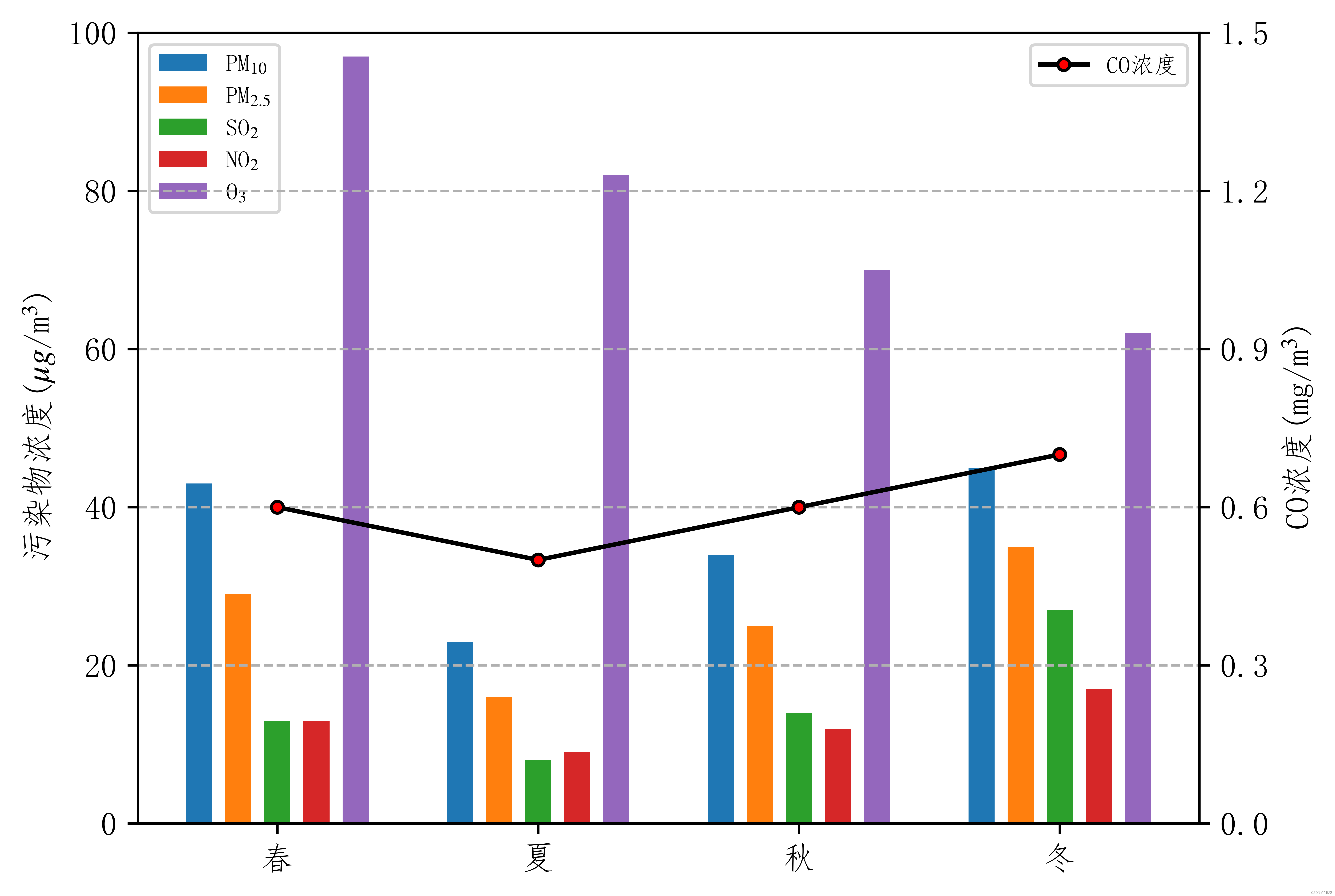
结果展示与分析

结果如下图所示，从该图可以看出各污染物季节平均浓度的变化趋势，有利于对该地区空气质量的各污染物季节变化变化情况有直观了解。最明显的就是臭氧浓度春夏季高、秋冬低，颗粒物浓度冬高夏低。

（图片右键新标签页打开会很清晰）

预告

下期进行污染物浓度月变化的分析。

以下是本人独自运营的微信公众号，用于分享个人学习及工作生活趣事，大佬们可以关注一波。