【PyTorch】迁移学习：基于 VGG 实现的光明哨兵与破败军团分类器

简述.

• 这是一个自我娱乐性质的小玩意儿，基础是迁移学习理论，数据集是人工收集的，尽力去保证训练集、验证集以及测试集分布大致相同。
• 光明哨兵和破败军团是 $\mathrm{M}\mathrm{o}\mathrm{b}\mathrm{a}$ 游戏英雄联盟 $\mathrm{L}\mathrm{e}\mathrm{a}\mathrm{g}\mathrm{u}\mathrm{e}\mathrm{o}\mathrm{f}\mathrm{L}\mathrm{e}\mathrm{g}\mathrm{e}\mathrm{n}\mathrm{d}\mathrm{s}$ 近期主线剧情的对立势力。两股势力中角色形象具有鲜明的特点，光明哨兵主要以光明、神圣的气质示人；而破败军团则相反，主旋律是压抑、阴沉。但由于角色背景故事中存在着黑化、飞升之类的设定，所以两股势力实际存在部分交集，简洁的说 —— 可能存在同一角色的不同时期属于不同类别。类似的问题实际在生物信息学中也存在，单细胞聚类中细胞的不同时期也会属于不同的聚类。

---

$\mathrm{V}\mathrm{G}\mathrm{G}$ 模型是 $2014$ 年 $\mathrm{I}\mathrm{L}\mathrm{S}\mathrm{V}\mathrm{R}\mathrm{C}$ 竞赛的第二名，第一名是 $\mathrm{G}\mathrm{o}\mathrm{o}\mathrm{g}\mathrm{L}\mathrm{e}\mathrm{N}\mathrm{e}\mathrm{t}.$ 但是 $\mathrm{V}\mathrm{G}\mathrm{G}$ 模型在多个迁移学习任务中的表现要优于 $\mathrm{G}\mathrm{o}\mathrm{o}\mathrm{g}\mathrm{L}\mathrm{e}\mathrm{N}\mathrm{e}\mathrm{t}.$ 而且，从图像中提取 $\mathrm{C}\mathrm{N}\mathrm{N}$ 特征，$\mathrm{V}\mathrm{G}\mathrm{G}$ 模型是首选算法。它的缺点在于，参数量有 $140\mathrm{M}$ 之多，需要更大的存储空间。但是这个模型很有研究价值。

• $\mathrm{V}\mathrm{G}\mathrm{G}16$ 是本次选用的迁移学习基础网络，在最后会对 $\mathrm{V}\mathrm{G}\mathrm{G}$ 做更加细致的介绍，$\mathrm{V}\mathrm{G}\mathrm{G}16$ 是在 $\mathrm{I}\mathrm{m}\mathrm{a}\mathrm{g}\mathrm{e}\mathrm{N}\mathrm{e}\mathrm{t}$ 上进行预训练的分类器，以识别 $1000$ 中物体类别。在 $\mathrm{P}\mathrm{y}\mathrm{T}\mathrm{o}\mathrm{r}\mathrm{c}\mathrm{h}-\mathrm{V}\mathrm{G}\mathrm{G}16$ 中，模型包含了两个部分 $\mathrm{f}\mathrm{e}\mathrm{a}\mathrm{t}\mathrm{u}\mathrm{r}\mathrm{e}\mathrm{s},\mathrm{c}\mathrm{l}\mathrm{a}\mathrm{s}\mathrm{s}\mathrm{i}\mathrm{f}\mathrm{i}\mathrm{e}\mathrm{r}\mathrm{s}$，前者是卷积网络部分，用于学习输入数据的特征；后者顾名思义是基于前部分学习到的特征进行分类。 一般进行迁移学习时，会冻结网络的卷积部分，对 $\mathrm{c}\mathrm{l}\mathrm{a}\mathrm{s}\mathrm{s}\mathrm{i}\mathrm{f}\mathrm{i}\mathrm{e}\mathrm{r}\mathrm{s}$ 做适当的修改，并进行参数学习。
• 数据集的组织方式按照 $\mathrm{P}\mathrm{y}\mathrm{T}\mathrm{o}\mathrm{r}\mathrm{c}\mathrm{h}-\mathrm{I}\mathrm{m}\mathrm{a}\mathrm{g}\mathrm{e}\mathrm{F}\mathrm{o}\mathrm{l}\mathrm{d}\mathrm{e}\mathrm{r}$ 的要求进行，即在训练集 $\mathrm{t}\mathrm{r}\mathrm{a}\mathrm{i}\mathrm{n}$、验证集 $\mathrm{v}\mathrm{a}\mathrm{l}\mathrm{i}\mathrm{d}$ 以及测试集 $\mathrm{t}\mathrm{e}\mathrm{s}\mathrm{t}$ 的文件夹下创建对应类别的图片文件夹，如下图所示：
  另外两个文件夹 $\mathrm{t}\mathrm{r}\mathrm{a}\mathrm{i}\mathrm{n},\mathrm{v}\mathrm{a}\mathrm{l}\mathrm{i}\mathrm{d}$ 的组织形式也相同。

---

环境配置.

• $\mathrm{S}\mathrm{p}\mathrm{y}\mathrm{d}\mathrm{e}\mathrm{r}5$
• $\mathrm{P}\mathrm{y}\mathrm{T}\mathrm{o}\mathrm{r}\mathrm{c}\mathrm{h}1.9.0$
• $\mathrm{P}\mathrm{y}\mathrm{t}\mathrm{h}\mathrm{o}\mathrm{n}3.8.8$

---

PyTorch代码.

• 下面分部分给出代码，并进行解释。在下文中，将光明哨兵 $\mathrm{S}\mathrm{e}\mathrm{n}\mathrm{t}\mathrm{i}\mathrm{n}\mathrm{e}\mathrm{l}\mathrm{s}-\mathrm{o}\mathrm{f}-\mathrm{L}\mathrm{i}\mathrm{g}\mathrm{h}\mathrm{t}$ 简记为 $\mathrm{s}\mathrm{o}\mathrm{l}$，破败军团 $\mathrm{R}\mathrm{u}\mathrm{i}\mathrm{n}\mathrm{e}\mathrm{d}$ 简记为 $\mathrm{r}\mathrm{u}\mathrm{i}.$

---

导入第三方库.

• 以 $\mathrm{P}\mathrm{y}\mathrm{T}\mathrm{o}\mathrm{r}\mathrm{c}\mathrm{h}$ 为主，另外 $\mathrm{M}\mathrm{a}\mathrm{t}\mathrm{p}\mathrm{l}\mathrm{o}\mathrm{t}\mathrm{l}\mathrm{i}\mathrm{b}$ 进行某些可视化展示。

# In[Import]
import torch
import torch.nn.functional as F
import torch.optim as optim
import matplotlib.pyplot as plt
import numpy as np
from torchvision import models
from torchvision import transforms
from torchvision.datasets import ImageFolder
from torch.utils.data import DataLoader

• $\mathrm{m}\mathrm{o}\mathrm{d}\mathrm{e}\mathrm{l}\mathrm{s}$ 中包含了预训练模型；$\mathrm{t}\mathrm{r}\mathrm{a}\mathrm{n}\mathrm{s}\mathrm{f}\mathrm{o}\mathrm{r}\mathrm{m}\mathrm{s}$ 用于完成归一化输入、数据增强处理过程。

---

使用 GPU.

• 判断 $\mathrm{G}\mathrm{P}\mathrm{U}$ 是否可用。

# In[GPU]
if torch.cuda.is_available():
    print('GPU works.')
    is_cuda = True

---

加载数据.

• 首先按照 $\mathrm{I}\mathrm{m}\mathrm{a}\mathrm{g}\mathrm{e}\mathrm{F}\mathrm{o}\mathrm{l}\mathrm{d}\mathrm{e}\mathrm{r}$ 读取数据，而后基于 $\mathrm{I}\mathrm{m}\mathrm{a}\mathrm{g}\mathrm{e}\mathrm{F}\mathrm{o}\mathrm{l}\mathrm{d}\mathrm{e}\mathrm{r}$ 构造 $\mathrm{D}\mathrm{a}\mathrm{t}\mathrm{a}\mathrm{L}\mathrm{o}\mathrm{a}\mathrm{d}\mathrm{e}\mathrm{r}.$

# In[DataSet]
simple_transform = \
    transforms.Compose([transforms.Resize((224,224)),
                        transforms.RandomHorizontalFlip(),
                        transforms.RandomRotation(0.2),
                        transforms.ToTensor(),
                        transforms.Normalize([0.485, 0.456, 0.406],
                                             [0.229, 0.224, 0.225])])
    
train = ImageFolder(r'D:/PythonCode/loldataset/train',
                    simple_transform)

valid = ImageFolder(r'D:/PythonCode/loldataset/valid',
                    simple_transform)
    
train_loader = DataLoader(train,
                          shuffle = True,
                          batch_size = 32,
                          num_workers = 0)

valid_loader = DataLoader(valid,
                          batch_size = 32,
                          num_workers = 0)

print('Train:',train.class_to_idx)
print('Valid:',valid.class_to_idx)

• 使用 $\mathrm{I}\mathrm{m}\mathrm{a}\mathrm{g}\mathrm{e}\mathrm{F}\mathrm{o}\mathrm{l}\mathrm{d}\mathrm{e}\mathrm{r}$ 读取数据集时要求路径指定的文件夹中，有标注数据是按照类别分文件夹存放的。

---

定义可视化函数.

• 由于图片读取后经历过处理 $\mathrm{s}\mathrm{i}\mathrm{m}\mathrm{p}\mathrm{l}\mathrm{e}\_\mathrm{t}\mathrm{r}\mathrm{a}\mathrm{n}\mathrm{s}\mathrm{f}\mathrm{o}\mathrm{r}\mathrm{m}$，从 $\mathrm{D}\mathrm{a}\mathrm{t}\mathrm{a}\mathrm{L}\mathrm{o}\mathrm{a}\mathrm{d}\mathrm{e}\mathrm{r}$ 中读取到数据后进行可视化是需要进行逆处理。

# In[Visual]
def myimshow(inputs):
    inputs = inputs.numpy().transpose((1,2,0))
    
    mean = np.array([0.485,0.456,0.406])
    std = np.array([0.229,0.224,0.225])
    
    inputs = inputs * std + mean
    inputs = np.clip(inputs,0,1)
    
    plt.imshow(inputs)
    
# In[Plot]
myimshow(train[34][0])

• 一个示例如下：
  
• 可以通过 $\mathrm{t}\mathrm{r}\mathrm{a}\mathrm{i}\mathrm{n}[34][1]$ 来查看其类别标签。

---

加载预训练模型.

• 代码会从网络上下载模型 $\mathrm{V}\mathrm{G}\mathrm{G}16$，第一次运行时下载速度可能较慢。完成下载后将模型加载到 $\mathrm{G}\mathrm{P}\mathrm{U}$ 上。

# In[VGG]
vgg = models.vgg16(pretrained = True)

if is_cuda:
    vgg = vgg.cuda()

---

冻结特征层.

• 如第一部分简述中所说，将 $\mathrm{V}\mathrm{G}\mathrm{G}16$ 中的卷积部分冻结，不改变预训练得到特征提取能力。

# In[Frozen]
for param in vgg.features.parameters():
    param.requires_grad = False

---

修改输出层.

• 由于 $\mathrm{V}\mathrm{G}\mathrm{G}16$ 是在 $K=1000$ 的数据集上训练的，而 $\mathrm{s}\mathrm{o}\mathrm{l}-\mathrm{r}\mathrm{u}\mathrm{i}$ 分类仅仅是二分类问题，所以需要对输出层进行修改。

# In[Output size]
'''Sentinel-of-Light & Ruined'''
vgg.classifier[6].out_features = 2

---

定义优化器.

• 这里选用带动量 $\mathrm{m}\mathrm{o}\mathrm{m}\mathrm{e}\mathrm{n}\mathrm{t}\mathrm{u}\mathrm{m}$ 的随机梯度下降法。

# In[Optimizer]
lr = 1e-2
momentum = 0.5
optimizer = optim.SGD(vgg.classifier.parameters(),lr = lr,
                      momentum = momentum)

---

定义训练函数.

# In[Fit function]
def fit(epoch,model,data_loader,phase = 'training'):
    if phase == 'training':
        model.train()
    if phase == 'validation':
        model.eval()
        
    run_loss = 0.0
    run_cor = 0
    
    for batch_id,(data,target) in enumerate(data_loader):
        if is_cuda:
            data,target = data.cuda(),target.cuda()
            
        if phase == 'training':
            optimizer.zero_grad()
            
        output = model(data)
        loss = F.cross_entropy(output,target)
        _,preds = torch.max(output.data,1)
        
        if phase == 'training':
            loss.backward()
            optimizer.step()
        
        run_loss = run_loss + loss.data
        run_cor = run_cor + torch.sum(preds == target.data)
        
        if phase == 'validation':
            print(np.where(preds != target))
        
    epoch_loss = run_loss/len(data_loader.dataset)
    epoch_acc = run_cor/len(data_loader.dataset)
    
    print(f'{phase} loss is {epoch_loss:{5}.{2}} and {phase} accuracy \\
    		is {run_cor}/{len(data_loader.dataset)} {epoch_acc:{10}.{4}}')

    return epoch_loss.cpu().numpy(),epoch_acc.cpu().numpy()

• $\mathrm{f}\mathrm{i}\mathrm{t}()$ 函数仅在 $\mathrm{t}\mathrm{r}\mathrm{a}\mathrm{i}\mathrm{n}\mathrm{i}\mathrm{n}\mathrm{g}$ 阶段才进行误差的反向传播和参数更新，在 $\mathrm{v}\mathrm{a}\mathrm{l}\mathrm{i}\mathrm{d}\mathrm{a}\mathrm{t}\mathrm{i}\mathrm{o}\mathrm{n}$ 阶段禁止使用该步骤。

---

训练过程.

• 将每个 $\mathrm{e}\mathrm{p}\mathrm{o}\mathrm{c}\mathrm{h}$ 训练的损失和准确率保存在列表中，后续用于绘制曲线，判断是否出现欠拟合、过拟合情况。

# In[Train]
train_losses,train_accuracy = [],[]
val_losses,val_accuracy = [],[]

epochs = 15

for epoch in range(epochs):
    epoch_loss,epoch_accuracy = fit(epoch,vgg,
                                     train_loader,
                                     phase='training')
    
    val_epoch_loss,val_epoch_accuracy = fit(epoch,vgg,
                                             valid_loader,
                                             phase='validation')
    train_losses.append(epoch_loss)
    train_accuracy.append(epoch_accuracy)
    val_losses.append(val_epoch_loss)
    val_accuracy.append(val_epoch_accuracy)  

• 一次训练的输出结果如下所示：

training loss is 0.0052 and training accuracy is 38/40       0.95
(array([5], dtype=int64),)
validation loss is 0.026 and validation accuracy is 9/10        0.9

training loss is 0.008 and training accuracy is 37/40      0.925
(array([1], dtype=int64),)
validation loss is 0.023 and validation accuracy is 9/10        0.9

training loss is 0.003 and training accuracy is 39/40      0.975
(array([1], dtype=int64),)
validation loss is 0.015 and validation accuracy is 9/10        0.9

training loss is 0.0019 and training accuracy is 40/40        1.0
(array([], dtype=int64),)
validation loss is 0.011 and validation accuracy is 10/10        1.0

training loss is 0.0011 and training accuracy is 39/40      0.975
(array([], dtype=int64),)
validation loss is 0.0093 and validation accuracy is 10/10        1.0

training loss is 0.00043 and training accuracy is 40/40        1.0
(array([1], dtype=int64),)
validation loss is 0.016 and validation accuracy is 9/10        0.9

training loss is 0.00091 and training accuracy is 40/40        1.0
(array([], dtype=int64),)
validation loss is  0.01 and validation accuracy is 10/10        1.0

training loss is 0.00056 and training accuracy is 40/40        1.0
(array([1], dtype=int64),)
validation loss is 0.013 and validation accuracy is 9/10        0.9

training loss is 0.0016 and training accuracy is 39/40      0.975
(array([], dtype=int64),)
validation loss is 0.011 and validation accuracy is 10/10        1.0

training loss is 0.0012 and training accuracy is 40/40        1.0
(array([], dtype=int64),)
validation loss is 0.0085 and validation accuracy is 10/10        1.0

training loss is 0.00068 and training accuracy is 40/40        1.0
(array([1], dtype=int64),)
validation loss is  0.01 and validation accuracy is 9/10        0.9

training loss is 0.00011 and training accuracy is 40/40        1.0
(array([1], dtype=int64),)
validation loss is 0.011 and validation accuracy is 9/10        0.9

training loss is 0.00033 and training accuracy is 40/40        1.0
(array([], dtype=int64),)
validation loss is 0.0064 and validation accuracy is 10/10        1.0

training loss is 0.001 and training accuracy is 40/40        1.0
(array([8], dtype=int64),)
validation loss is 0.012 and validation accuracy is 9/10        0.9

training loss is 0.0038 and training accuracy is 39/40      0.975
(array([1], dtype=int64),)
validation loss is 0.011 and validation accuracy is 9/10        0.9

• 实际上可以发现，验证损失是在波动的，因此可以适当减少 $\mathrm{e}\mathrm{p}\mathrm{o}\mathrm{c}\mathrm{h}\mathrm{s}.$ 最后发现测试集中的 $1$ 号图片预测错误，这里将图片展示如下：
  
• 这张是破败之王被动技能的图标，归于 $\mathrm{R}\mathrm{u}\mathrm{i}\mathrm{n}\mathrm{e}\mathrm{d}$ 类别中。
• 【补充】后续将 $\mathrm{e}\mathrm{p}\mathrm{o}\mathrm{c}\mathrm{h}\mathrm{s}$ 降低到 $8$，重新训练后的结果如下：

training loss is  0.35 and training accuracy is 3/40      0.075
(array([1, 7, 8, 9], dtype=int64),)
validation loss is  0.12 and validation accuracy is 6/10        0.6

training loss is 0.032 and training accuracy is 30/40       0.75
(array([5, 8], dtype=int64),)
validation loss is 0.073 and validation accuracy is 8/10        0.8

training loss is 0.0098 and training accuracy is 35/40      0.875
(array([], dtype=int64),)
validation loss is 0.011 and validation accuracy is 10/10        1.0

training loss is 0.0045 and training accuracy is 39/40      0.975
(array([], dtype=int64),)
validation loss is 0.013 and validation accuracy is 10/10        1.0

training loss is 0.001 and training accuracy is 40/40        1.0
(array([], dtype=int64),)
validation loss is 0.011 and validation accuracy is 10/10        1.0

training loss is 0.00077 and training accuracy is 40/40        1.0
(array([], dtype=int64),)
validation loss is 0.012 and validation accuracy is 10/10        1.0

training loss is 0.002 and training accuracy is 39/40      0.975
(array([], dtype=int64),)
validation loss is 0.0079 and validation accuracy is 10/10        1.0

training loss is 0.00025 and training accuracy is 40/40        1.0
(array([], dtype=int64),)
validation loss is 0.008 and validation accuracy is 10/10        1.0

• $\mathrm{e}\mathrm{p}\mathrm{o}\mathrm{c}\mathrm{h}\mathrm{s}=8$ 的测试情况如下所示：

Test: {'rui': 0, 'sol': 1}
(array([1], dtype=int64),)
validation loss is 0.023 and validation accuracy is 15/16     0.9375

---

绘制损失、准确率曲线.

• 根据上面 $\mathrm{e}\mathrm{p}\mathrm{o}\mathrm{c}\mathrm{h}\mathrm{s}=15$ 得到的损失以及准确率，进行曲线绘制，直观地判断拟合情况。

# In[Plot loss]
plt.plot(range(1,len(train_losses)+1),
         train_losses,'bo',
         label = 'training loss')
plt.plot(range(1,len(val_losses)+1),
         val_losses,'r',
         label = 'validation loss')
plt.legend()

# In[Plot acc]
plt.plot(range(1,len(train_accuracy)+1),
         train_accuracy,'bo',
         label = 'train accuracy')
plt.plot(range(1,len(val_accuracy)+1),
         val_accuracy,'r',
         label = 'val accuracy')
plt.legend()   

• 得到的曲线如下图所示：
  
  

---

测试情况.

• 最后给出 $\mathrm{e}\mathrm{p}\mathrm{o}\mathrm{c}\mathrm{h}\mathrm{s}=15$ 训练得到的模型，在测试集上进行模型的预测，并查看预测错误的样本。

# In[Test]
test = ImageFolder(r'D:/PythonCode/loldataset/test',simple_transform)
print('Test:',test.class_to_idx)
    
test_loader = DataLoader(test,batch_size = 32,num_workers = 0)
    
test_loss,test_acc = fit(1,vgg,test_loader,phase='validation')

• 打印出的信息如下：

Test: {'rui': 0, 'sol': 1}
(array([1, 2], dtype=int64),)
validation loss is 0.027 and validation accuracy is 14/16      0.875

• 其中索引号为 $1,2$ 的样本预测错误，展示如下：
  
• 上图是破败小小英雄，将其放入测试集中确是有 “为难” $\mathrm{s}\mathrm{o}\mathrm{l}-\mathrm{r}\mathrm{u}\mathrm{i}$ 分类器的目的。另一张预测错误的图片如下：
  
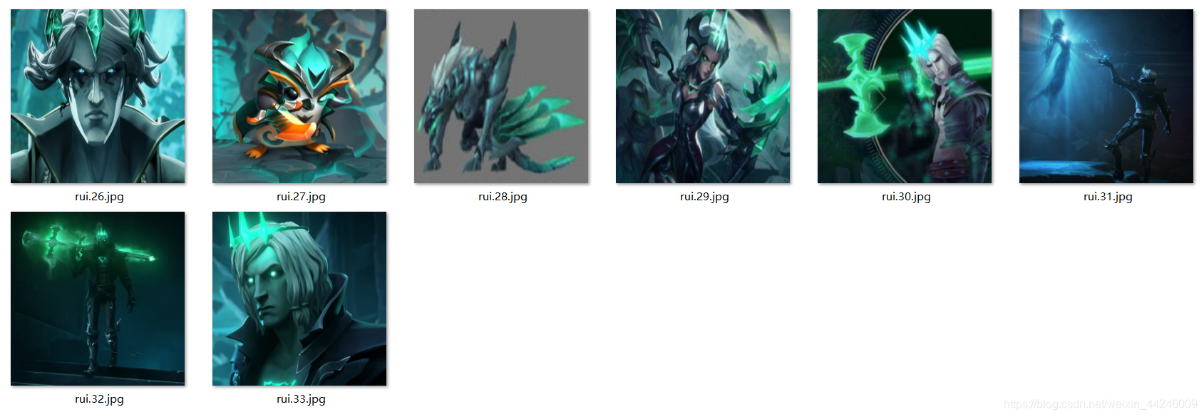
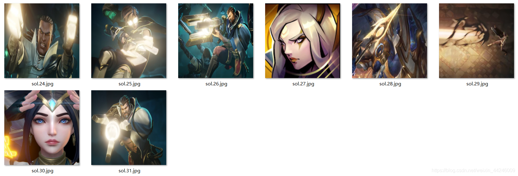
• 上图是破败龙女大招的形态，但其属于破败军团的特征应该是比较明显的，注意到 $\mathrm{e}\mathrm{p}\mathrm{o}\mathrm{c}\mathrm{h}\mathrm{s}=15$ 的训练过程中是存在验证损失增高情况的，需要调整训练过程。整个测试集的缩略图如下：
  
  

---

可视化中间层激活状态.

• 对中间层的激活状态进行可视化有助于我们理解图像数据在各层之间的变化情况，从侧面反映出不同卷积层关注的重点。默认情况下，$\mathrm{P}\mathrm{y}\mathrm{T}\mathrm{o}\mathrm{r}\mathrm{c}\mathrm{h}$ 为了降低内存占用，只会保存模型最后一层的输出，因此我们需要借助其他手段提取中间层的激活状态。
• $\mathrm{P}\mathrm{y}\mathrm{T}\mathrm{o}\mathrm{r}\mathrm{c}\mathrm{h}$ 提供了一个名为 $\mathrm{r}\mathrm{e}\mathrm{g}\mathrm{i}\mathrm{s}\mathrm{t}\mathrm{e}\mathrm{r}\_\mathrm{f}\mathrm{o}\mathrm{r}\mathrm{w}\mathrm{a}\mathrm{r}\mathrm{d}\_\mathrm{h}\mathrm{o}\mathrm{o}\mathrm{k}$ 的函数，它允许传入一个完成提取特定层输出的函数。可视化中间层激活状态的代码如下所示：

# In[Activate]
class LayerActivations():
    features = None

    def __init__(self,model,layer):
        self.hook = \
            model[layer].register_forward_hook(self.hook_fn)

    def hook_fn(self,module,inputs,output):
        self.features = output.cpu()
        
    def remove(self):
        self.hook.remove()

• 选择某张图片 $\mathrm{i}\mathrm{m}\mathrm{g}$ 后，查看它在不同卷积层中的输出。$\mathrm{i}\mathrm{m}\mathrm{g}$ 原图如下，是一张很猖狂的德莱文：
  
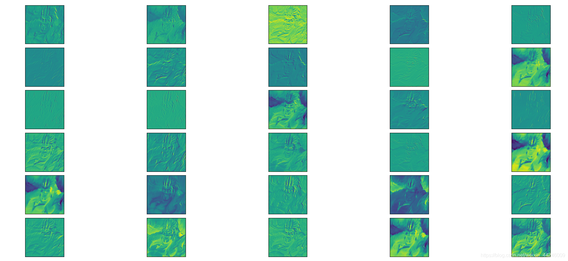
• 第一个卷积层的输出如下所示：
  
• 可以看出是在检测一些线条和边缘，较浅卷积层的输出大抵都是如此：
  
  
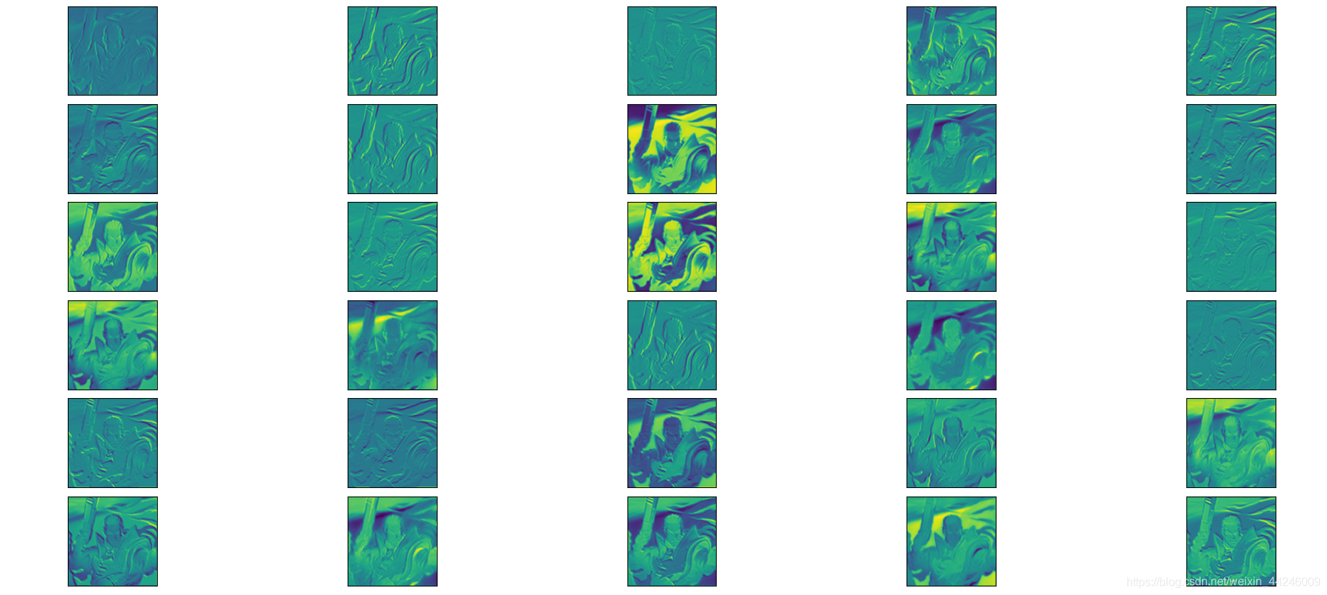
• 下图是卢锡安在第 $7$ 卷积层 ( 对应 $\mathrm{l}\mathrm{a}\mathrm{y}\mathrm{e}\mathrm{r}$ 是 $14$ ) 中的输出，可以发现深层是在学习更加抽象的特征：
  
• 一般来说，$\mathrm{C}\mathrm{N}\mathrm{N}$ 的前几层专注于较小的特征，例如线条和曲线的外观；而更深层次的卷积核识别更高级的特征，例如猫狗分类识别时学习到的眼睛、鼻子等。选择预训练模型时需要注意数据集的相似性，$\mathrm{I}\mathrm{m}\mathrm{a}\mathrm{g}\mathrm{e}\mathrm{N}\mathrm{e}\mathrm{t}$ 数据集中有 $1000$ 种类别，因此我们这里的 $\mathrm{V}\mathrm{G}\mathrm{G}16$ 具有能够识别多种模式的卷积核权重，在进行 $\mathrm{s}\mathrm{o}\mathrm{l}-\mathrm{r}\mathrm{u}\mathrm{i}$ 分类器训练时保持卷积层提取特征的能力不变，学习线性层分类权重即可获得很好的效果。

---

VGG16.

• $\mathrm{V}\mathrm{G}\mathrm{G}16$ 架构包含 $5$ 个 $\mathrm{V}\mathrm{G}\mathrm{G}$ 块，一个 $\mathrm{V}\mathrm{G}\mathrm{G}$ 块由一组卷积层及其非线性激活函数与一个最大池化层组成。可以打印出 $\mathrm{V}\mathrm{G}\mathrm{G}16$ 的架构信息：

VGG(
  (features): Sequential(
    (0): Conv2d(3, 64, kernel_size=(3, 3), stride=(1, 1), padding=(1, 1))
    (1): ReLU(inplace=True)
    (2): Conv2d(64, 64, kernel_size=(3, 3), stride=(1, 1), padding=(1, 1))
    (3): ReLU(inplace=True)
    (4): MaxPool2d(kernel_size=2, stride=2, padding=0, dilation=1, ceil_mode=False)
    
    (5): Conv2d(64, 128, kernel_size=(3, 3), stride=(1, 1), padding=(1, 1))
    (6): ReLU(inplace=True)
    (7): Conv2d(128, 128, kernel_size=(3, 3), stride=(1, 1), padding=(1, 1))
    (8): ReLU(inplace=True)
    (9): MaxPool2d(kernel_size=2, stride=2, padding=0, dilation=1, ceil_mode=False)
    
    (10): Conv2d(128, 256, kernel_size=(3, 3), stride=(1, 1), padding=(1, 1))
    (11): ReLU(inplace=True)
    (12): Conv2d(256, 256, kernel_size=(3, 3), stride=(1, 1), padding=(1, 1))
    (13): ReLU(inplace=True)
    (14): Conv2d(256, 256, kernel_size=(3, 3), stride=(1, 1), padding=(1, 1))
    (15): ReLU(inplace=True)
    (16): MaxPool2d(kernel_size=2, stride=2, padding=0, dilation=1, ceil_mode=False)
    
    (17): Conv2d(256, 512, kernel_size=(3, 3), stride=(1, 1), padding=(1, 1))
    (18): ReLU(inplace=True)
    (19): Conv2d(512, 512, kernel_size=(3, 3), stride=(1, 1), padding=(1, 1))
    (20): ReLU(inplace=True)
    (21): Conv2d(512, 512, kernel_size=(3, 3), stride=(1, 1), padding=(1, 1))
    (22): ReLU(inplace=True)
    (23): MaxPool2d(kernel_size=2, stride=2, padding=0, dilation=1, ceil_mode=False)
    
    (24): Conv2d(512, 512, kernel_size=(3, 3), stride=(1, 1), padding=(1, 1))
    (25): ReLU(inplace=True)
    (26): Conv2d(512, 512, kernel_size=(3, 3), stride=(1, 1), padding=(1, 1))
    (27): ReLU(inplace=True)
    (28): Conv2d(512, 512, kernel_size=(3, 3), stride=(1, 1), padding=(1, 1))
    (29): ReLU(inplace=True)
    (30): MaxPool2d(kernel_size=2, stride=2, padding=0, dilation=1, ceil_mode=False)
  )
  (avgpool): AdaptiveAvgPool2d(output_size=(7, 7))
  (classifier): Sequential(
    (0): Linear(in_features=25088, out_features=4096, bias=True)
    (1): ReLU(inplace=True)
    (2): Dropout(p=0.5, inplace=False)
    (3): Linear(in_features=4096, out_features=4096, bias=True)
    (4): ReLU(inplace=True)
    (5): Dropout(p=0.5, inplace=False)
    (6): Linear(in_features=4096, out_features=2, bias=True)
  )
)

---

完整代码.

• 由于编码时使用 $\mathrm{S}\mathrm{p}\mathrm{y}\mathrm{d}\mathrm{e}\mathrm{r}$ 的 $\mathrm{c}\mathrm{e}\mathrm{l}\mathrm{l}$ 运行方式，因此直接运行整个 $.\mathrm{p}\mathrm{y}$ 文件会导致很多中间结果的图片展示混乱，建议采用 $\mathrm{S}\mathrm{p}\mathrm{y}\mathrm{d}\mathrm{e}\mathrm{r}$ 或 $\mathrm{j}\mathrm{u}\mathrm{p}\mathrm{y}\mathrm{t}\mathrm{e}\mathrm{r}\mathrm{n}\mathrm{o}\mathrm{t}\mathrm{e}\mathrm{b}\mathrm{o}\mathrm{o}\mathrm{k}$ 体验。

# In[Import]
import torch
import torch.nn.functional as F
import torch.optim as optim
import matplotlib.pyplot as plt
import numpy as np
from torchvision import models
from torchvision import transforms
from torchvision.datasets import ImageFolder
from torch.utils.data import DataLoader

# In[GPU]
if torch.cuda.is_available():
    print('GPU works.')
    is_cuda = True
    
# In[DataSet]
simple_transform = \
    transforms.Compose([transforms.Resize((224,224)),
                        transforms.RandomHorizontalFlip(),
                        transforms.RandomRotation(0.2),
                        transforms.ToTensor(),
                        transforms.Normalize([0.485, 0.456, 0.406],
                                             [0.229, 0.224, 0.225])])
    
train = ImageFolder(r'D:/PythonCode/loldataset/train',
                    simple_transform)

valid = ImageFolder(r'D:/PythonCode/loldataset/valid',
                    simple_transform)
    
train_loader = DataLoader(train,
                          shuffle = True,
                          batch_size = 32,
                          num_workers = 0)

valid_loader = DataLoader(valid,
                          batch_size = 32,
                          num_workers = 0)

print('Train:',train.class_to_idx)
print('Valid:',valid.class_to_idx)

# In[Visual]
def myimshow(inputs):
    inputs = inputs.numpy().transpose((1,2,0))
    
    mean = np.array([0.485,0.456,0.406])
    std = np.array([0.229,0.224,0.225])
    
    inputs = inputs * std + mean
    inputs = np.clip(inputs,0,1)
    
    plt.imshow(inputs)
    
# In[Plot]
myimshow(train[2][0])
    
# In[VGG]
vgg = models.vgg16(pretrained = True)

if is_cuda:
    vgg = vgg.cuda()
 
# In[Frozen]
for param in vgg.features.parameters():
    param.requires_grad = False
    
# In[Output size]
'''Sentinel-of-Light & Ruined'''
vgg.classifier[6].out_features = 2
    
# In[Optimizer]
lr = 1e-2
momentum = 0.5
optimizer = optim.SGD(vgg.classifier.parameters(),
                      lr = lr,
                      momentum = momentum)
    
# In[Fit function]
def fit(epoch,model,data_loader,phase = 'training'):
    if phase == 'training':
        model.train()
    if phase == 'validation':
        model.eval()
        
    run_loss = 0.0
    run_cor = 0
    
    for batch_id,(data,target) in enumerate(data_loader):
        if is_cuda:
            data,target = data.cuda(),target.cuda()
            
        if phase == 'training':
            optimizer.zero_grad()
            
        output = model(data)
        loss = F.cross_entropy(output,target)
        _,preds = torch.max(output.data,1)
        
        if phase == 'training':
            loss.backward()
            optimizer.step()
        
        run_loss = run_loss + loss.data
        run_cor = run_cor + torch.sum(preds == target.data)
        
        if phase == 'validation':
            print(np.where(preds.cpu().numpy() != target.data.cpu().numpy()))
        
    epoch_loss = run_loss/len(data_loader.dataset)
    epoch_acc = run_cor/len(data_loader.dataset)
    
    print(f'{phase} loss is {epoch_loss:{5}.{2}} and {phase} accuracy \\
    	is {run_cor}/{len(data_loader.dataset)} {epoch_acc:{10}.{4}}')

    return epoch_loss.cpu().numpy(),epoch_acc.cpu().numpy()

# In[Train]
train_losses,train_accuracy = [],[]
val_losses,val_accuracy = [],[]

epochs = 8

for epoch in range(epochs):
    epoch_loss,epoch_accuracy = fit(epoch,vgg,
                                     train_loader,
                                     phase='training')
    
    val_epoch_loss,val_epoch_accuracy = fit(epoch,vgg,
                                             valid_loader,
                                             phase='validation')
    train_losses.append(epoch_loss)
    train_accuracy.append(epoch_accuracy)
    val_losses.append(val_epoch_loss)
    val_accuracy.append(val_epoch_accuracy)        

# In[Plot loss]
plt.plot(range(1,len(train_losses)+1),
         train_losses,'bo',
         label = 'training loss')
plt.plot(range(1,len(val_losses)+1),
         val_losses,'r',
         label = 'validation loss')
plt.legend()

# In[Plot acc]
plt.plot(range(1,len(train_accuracy)+1),
         train_accuracy,'bo',
         label = 'train accuracy')
plt.plot(range(1,len(val_accuracy)+1),
         val_accuracy,'r',
         label = 'val accuracy')
plt.legend()   
    
# In[Test]
test = ImageFolder(r'D:/PythonCode/loldataset/test',
                    simple_transform)

print('Test:',test.class_to_idx)
    
test_loader = DataLoader(test,
                         batch_size = 32,
                         num_workers = 0)
    
test_loss,test_acc = fit(1,vgg,test_loader,phase='validation')

# In[Activate]
class LayerActivations():
    features = None

    def __init__(self,model,layer):
        self.hook = \
            model[layer].register_forward_hook(self.hook_fn)

    def hook_fn(self,module,inputs,output):
        self.features = output.cpu()
        
    def remove(self):
        self.hook.remove()

# In[Sample img]
img = next(iter(train_loader))[0]

# In[Plot]
layer = 14

conv_out = LayerActivations(vgg.features, layer)
o = vgg(img.cuda())
conv_out.remove()

act = conv_out.features

fig = plt.figure(figsize = (20,50))
fig.subplots_adjust(left = 0,
                    right = 1,
                    bottom = 0.1,
                    top = 0.9,
                    hspace = 0.1,
                    wspace = 0.1)

for i in range(30):
    ax = fig.add_subplot(6,5,i+1,xticks = [],yticks = [])
    ax.imshow(act[0][i])

---