


记录TensorFlow听课笔记
文章目录
*[参考博文](%E5%8E%9F%E6%96%87%E9%93%BE%E6%8E%A5%EF%BC%9Ahttps://blog.csdn.net/qq_42604176/article/details/108282705)*
一,线性回归
将自变量和因变量之间的关系,用线性模型来表示 根据已知的样本数据,对未来的、或者未知的数据进行估计。

二,广义线性回归

分类问题:垃圾邮件识别、图片分类、疾病判断
分类器:能够自动对输入的数据进行分类 输入:特征,输出:离散值

实现分类器:
准备训练样本
训练分类器
对新样本分类
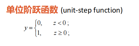
激活函数

对数几率函数(logistic function)

对数几率回归/逻辑回归(logistic regression)
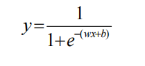
Sigmoid函数
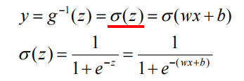
多元模型

损失函数
线性回归的处理值是连续值,不适合处理分类任务
用sigmoid函数,将线性回归的返回值映射到(0,1)之间的概率值,然后设定阈值,实现分类
sigmoid函数大部分比较平缓,导数值较小,这导致了参数迭代更新缓慢
在线性回归中平方损失函数是一个凸函数,只有一个极小值点
但是在逻辑回归中,它的平方损失函数是一个非凸函数,有许多局部极小值点,使用梯度下降法可能得到的知识局部极小值
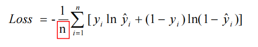
所以,在逻辑回归中一般使用交叉熵损失函数(联系统计学中的极大似然估计)
平方损失函数

交叉熵损失函数

平均交叉熵损失函数


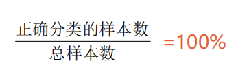
准确率 (accuracy):

三,一元/多元逻辑回归

numpy实现sigmoid()函数

numpy实现交叉熵损失函数

numpy方法得到准确率


四,实现一元逻辑回归
#实现一元逻辑回归
import tensorflow as tf
import numpy as np
import matplotlib.pyplot as plt

x=np.array([137.97,104.50,100.00,126.32,79.20,99.00,124.00,114.00,106.69,140.05,53.75,46.91,68.00,63.02,81.26,86.21])
y=np.array([1,1,0,1,0,1,1,0,0,1,0,0,0,0,0,0])
#plt.scatter(x,y)
#中心化操作,使得中心点为0
x_train=x-np.mean(x)
y_train=y
plt.scatter(x_train,y_train)
#设置超参数
learn_rate=0.005
#迭代次数
iter=5
#每10次迭代显示一下效果
display_step=1
#设置模型参数初始值
np.random.seed(612)
w=tf.Variable(np.random.randn())
b=tf.Variable(np.random.randn())
#观察初始参数模型
x_start=range(-80,80)
y_start=1/(1+tf.exp(-(w*x_start+b)))
plt.plot(x_start,y_start,color="red",linewidth=3)
#训练模型
#存放训练集的交叉熵损失、准确率
cross_train=[]
acc_train=[]
for i in range(0,iter+1):
    with tf.GradientTape() as tape:
        #sigmoid函数
        pred_train=1/(1+tf.exp(-(w*x_train+b)))
        #交叉熵损失函数
        Loss_train=-tf.reduce_mean(y_train*tf.math.log(pred_train)+(1-y_train)*tf.math.log(1-pred_train))
        #训练集准确率
        Accuracy_train=tf.reduce_mean(tf.cast(tf.equal(tf.where(pred_train<0.5,0,1),y_train),tf.float32))
    #记录每一次迭代的损失和准确率
    cross_train.append(Loss_train)
    acc_train.append(Accuracy_train)
    #更新参数
    dL_dw,dL_db = tape.gradient(Loss_train,[w,b])
    w.assign_sub(learn_rate*dL_dw)
    b.assign_sub(learn_rate*dL_db)
    #plt.plot(x,pred)
    if i % display_step==0:
        print("i:%i, Train Loss:%f,Accuracy:%f"%(i,cross_train[i],acc_train[i]))
        y_start=1/(1+tf.exp(-(w*x_start+b)))
        plt.plot(x_start,y_start)

#进行分类,并不是测试集,测试集是有标签的数据,而我们这边没有标签,这里是真实场景的应用情况
#商品房面积
x_test=[128.15,45.00,141.43,106.27,99.00,53.84,85.36,70.00,162.00,114.60]
#根据面积计算概率,这里使用训练数据的平均值进行中心化处理
pred_test=1/(1+tf.exp(-(w*(x_test-np.mean(x))+b)))
#根据概率进行分类
y_test=tf.where(pred_test<0.5,0,1)
#打印数据
for i in range(len(x_test)):
    print(x_test[i],"\t",pred_test[i].numpy(),"\t",y_test[i].numpy(),"\t")
#可视化输出
plt.figure()
plt.scatter(x_test,y_test)
x_=np.array(range(-80,80))
y_=1/(1+tf.exp(-(w*x_+b)))
plt.plot(x_+np.mean(x),y_)
plt.show()

五,多分类问题


二分类的模型参数是一个列向量W(n+1行)
多分类的模型参数是一个矩阵W(n+1行,n+1列)
这里使用softmax回归(而不是对数几率函数)。
softmax回归:适用于样本的标签互斥的情况。比如,样本的标签为,房子,小车和自行车,这三类之间是没有关系的。样本只能是属于其中一个标签。
逻辑回归:使用于样本的标签有重叠的情况。比如:外套,大衣和毛衣,一件衣服可以即属于大衣,由属于外套。这个时候就需要三个独立的逻辑回归模型。


六,TensorFlow实现多分类问题
逻辑回归只能解决二分类问题
独热编码
a=[0,2,3,5]
#独热编码
#one_hot(一维数组/张量,编码深度)
b=tf.one_hot(a,6)
print(b)
结果
tf.Tensor(
[[1. 0. 0. 0. 0. 0.]
 [0. 0. 1. 0. 0. 0.]
 [0. 0. 0. 1. 0. 0.]
 [0. 0. 0. 0. 0. 1.]], shape=(4, 6), dtype=float32)
计算准确率
导入预测值
导入标记
将标记独热编码
获取预测值中的最大数索引
判断预测值是否与样本标记是否相同
上个步骤判断结果的将布尔值转化为数字
计算准确率
#准确率

#预测值
pred=np.array([[0.1,0.2,0.7],
               [0.1,0.7,0.2],
               [0.3,0.4,0.3]])
#标记
y=np.array([2,1,0])
#标记独热编码
y_onehot=np.array([[0,0,1],[0,1,0],[1,0,0]])

#预测值中的最大数索引
print(tf.argmax(pred,axis=1))
#判断预测值是否与样本标记是否相同
print(tf.equal(tf.argmax(pred,axis=1),y))
#将布尔值转化为数字
print(tf.cast(tf.equal(tf.argmax(pred,axis=1),y),tf.float32))
#计算准确率
print(tf.reduce_mean(tf.cast(tf.equal(tf.argmax(pred,axis=1),y),tf.float32)))
结果
tf.Tensor([2 1 1], shape=(3,), dtype=int64)
tf.Tensor([ True  True False], shape=(3,), dtype=bool)
tf.Tensor([1. 1. 0.], shape=(3,), dtype=float32)
tf.Tensor(0.6666667, shape=(), dtype=float32)
计算交叉熵损失函数
#交叉损失函数
#计算样本交叉熵
print(-y_onehot*tf.math.log(pred))
#计算所有样本交叉熵之和
print(-tf.reduce_sum(-y_onehot*tf.math.log(pred)))
#计算平均交叉熵损失
print(-tf.reduce_sum(-y_onehot*tf.math.log(pred))/len(pred))
结果
tf.Tensor(
[[-0.         -0.          0.35667494]
 [-0.          0.35667494 -0.        ]
 [ 1.2039728  -0.         -0.        ]], shape=(3, 3), dtype=float64)
tf.Tensor(-1.917322692203401, shape=(), dtype=float64)
tf.Tensor(-0.6391075640678003, shape=(), dtype=float64)
七,使用花瓣长度、花瓣宽度将三种鸢尾花区分开
import tensorflow as tf
import pandas as pd
import numpy as np
import matplotlib as mpl
import matplotlib.pyplot as plt

#=============================加载数据============================================
#下载鸢尾花数据集iris
#训练数据集 120条数据
#测试数据集 30条数据
import tensorflow as tf
TRAIN_URL = "http://download.tensorflow.org/data/iris_training.csv"
train_path = tf.keras.utils.get_file(TRAIN_URL.split('/')[-1],TRAIN_URL)

df_iris_train = pd.read_csv(train_path,header=0)
#=============================处理数据============================================
iris_train = np.array(df_iris_train)
#观察形状
print(iris_train.shape)
#提取花瓣长度、花瓣宽度属性
x_train=iris_train[:,2:4]
#提取花瓣标签
y_train=iris_train[:,4]
print(x_train.shape,y_train)
num_train=len(x_train)
x0_train =np.ones(num_train).reshape(-1,1)
X_train =tf.cast(tf.concat([x0_train,x_train],axis=1),tf.float32)
Y_train =tf.one_hot(tf.constant(y_train,dtype=tf.int32),3)

print(X_train.shape,Y_train)

#=============================设置超参数、设置模型参数初始值============================================
learn_rate=0.2
#迭代次数
iter=500
#每10次迭代显示一下效果
display_step=100
np.random.seed(612)
W=tf.Variable(np.random.randn(3,3),dtype=tf.float32)
#=============================训练模型============================================
#存放训练集准确率、交叉熵损失
acc=[]
cce=[]
for i in range(0,iter+1):
    with tf.GradientTape() as tape:
        PRED_train=tf.nn.softmax(tf.matmul(X_train,W))
        #计算CCE
        Loss_train=-tf.reduce_sum(Y_train*tf.math.log(PRED_train))/num_train
    #计算啊准确度
    accuracy=tf.reduce_mean(tf.cast(tf.equal(tf.argmax(PRED_train.numpy(),axis=1),y_train),tf.float32))
    acc.append(accuracy)
    cce.append(Loss_train)
    #更新参数
    dL_dW = tape.gradient(Loss_train,W)
    W.assign_sub(learn_rate*dL_dW)
    #plt.plot(x,pred)
    if i % display_step==0:
        print("i:%i, Acc:%f,CCE:%f"%(i,acc[i],cce[i]))

#观察训练结果
print(PRED_train.shape)
#相加之后概率和应该为1
print(tf.reduce_sum(PRED_train,axis=1))
#转换为自然顺序编码
print(tf.argmax(PRED_train.numpy(),axis=1))

#绘制分类图
#设置图的大小
M=500
x1_min,x2_min =x_train.min(axis=0)
x1_max,x2_max =x_train.max(axis=0)
#在闭区间[min,max]生成M个间隔相同的数字
t1 =np.linspace(x1_min,x1_max,M)
t2 =np.linspace(x2_min,x2_max,M)
m1,m2 =np.meshgrid(t1,t2)

m0=np.ones(M*M)
#堆叠数组S
X_ =tf.cast(np.stack((m0,m1.reshape(-1),m2.reshape(-1)),axis=1),tf.float32)
Y_ =tf.nn.softmax(tf.matmul(X_,W))
#转换为自然顺序编码,决定网格颜色
Y_ =tf.argmax(Y_.numpy(),axis=1)
n=tf.reshape(Y_,m1.shape)
plt.figure(figsize=(8,6))
cm_bg =mpl.colors.ListedColormap(['#A0FFA0','#FFA0A0','#A0A0FF'])
plt.pcolormesh(m1,m2,n,cmap=cm_bg)
plt.scatter(x_train[:,0],x_train[:,1],c=y_train,cmap="brg")
plt.show()


 被折叠的 条评论
为什么被折叠?
被折叠的 条评论
为什么被折叠?
 到【灌水乐园】发言


