pytorch-12 深度学习基础网络的数据集创建及手动搭建实现

白白白飘

已于 2024-05-24 01:48:18 修改

阅读量665

点赞数 19

分类专栏：深度学习神经网络Pytorch 文章标签：深度学习 pytorch 人工智能

于 2024-05-12 23:37:33 首次发布

本文链接：https://blog.csdn.net/weixin_45311418/article/details/138716706

版权

深度学习神经网络Pytorch 专栏收录该内容

10 篇文章 0 订阅

订阅专栏

Lesson 12. 前言

尽管深度学习也属于机器学习范畴，基本的建模理念和机器学习类似，比如需要确定目标函数和损失函数、找到合适的优化算法对参数进行求解等等，但利用PyTorch在进行建模的过程却和和最大的机器学习库Scikit-Learn中定义的机器学习建模方法有较大的差别。

在数据读取过程中，PyTorch需要将数据先封装在一个Dataset的子类里面，然后再用DataLoader进行装载，然后才能带入训练，而sklearn则可以直接读取Pandas中存储的面板数据进行建模；
在模型调用的过程，PyTorch需要先创建一个Module的子类去定义模型基本结构，然后才能实例化这个模型进行训练，并且训练过程中优化算法也是某个类的实例化结果，在训练过程中需要实用这个类的诸多方法来将梯度清零或者更新神经元之间连接的权重。相比之下sklearn则简单的多，只需要在实例化模型的过程中定义好超参数的取值，然后实用fit方法进行训练即可。

那为何PyTorch的整个实现过程看似会更加复杂？归根结底，还是和深度学习建模的特殊性有关。
类似PyTorch的这种，看似对初学者略显复杂的建模流程，实际上都是为了能够更好的满足深度学习建模的一般情况：针对非结构化数据、在超大规模的数据集上进行模型训练。

PyTorch在读取数据的过程中需要使用Dataset和DataLoader数据进行封装和加载，其实是为了能够实现数据的迭代式存储和映射式存储，也就是通过生成数据的生成器或者保存数据的映射关系，来避免数据的重复存储
如进行小批量数据划分时，PyTorch并未真正意义上的把数据进行切分然后单独存储，而是创建了每个“小批”数据和原数据的映射关系（或者说“小批”数据的索引值），然后借助这种映射关系，在实际需要使用这些数据的时候在对其进行提取。因为当进行海量数据处理时，划分多个数据集进行额外的存储显然是不合适的。

但不管怎样，这样的一个建模流程还是给很多初学者造成一定的学习难度，然而熟练掌握深度学习建模流程、熟练使用基本函数和类却是后续学习的基础，因此，在正式进入到下个阶段之前，也就是正式进入到深度学习优化算法学习之前，我们需要进行一段时间的强化练习，通过对此前介绍的基础神经网络进行手动建模实现和调库实现，强化代码能力。
此外，在前几节课的学习当中我们也发现，PyTorch作为新兴的深度学习计算框架，在某些功能实现上还显得不够完善，比如此前我们看到的将“概率”结果划为类别判别的过程、准确率计算过程等等，PyTorch中都没有提供原生的函数作为支持，因此我们需要手动编写此类实用函数。外加模型训练过程本身也可以封装在函数内，因此本节我们也将手动编写PyTorch实际应用中的实用函数作为nn.functional的补充。
另外，为了在后续的优化算法部分课程中更好的观察模型不同优化算法能够起到的作用，本节课程还将介绍数据集创建函数、模型可视化工具TensorBoard安装和实用方法；同时，虽然是建模练习，但可能会涉及一定规模的运算，因此我们还将在本节还将介绍模型的GPU运行方法。

# 导包
import random
import matplotlib as mpl
from matplotlib import pyplot
import matplotlib.pyplot as plt
import numpy as np

import torch
from torch import nn,optim
import torch.nn.functional as F
from torch.utils.data import Dataset,TensorDataset,DataLoader

# 自定义模块
from torchLearning import *

# 导入以下包从而使得可以在jupyter中的一个cell输出多个结果
from IPython.core.interactiveshell import InteractiveShell
InteractiveShell.ast_node_interactivity = "all"

Lesson 12.1 数据集创建函数

1、回归类数据集手动创建方法

回归类模型的数据，特征和标签都是连续型数值。（1）生成两个特征、存在偏差，自变量和因变量存在线性关系的数据集（2）生成非线性关系的数据集，此处我们创建满足 $y=x^2+1$ 规律的数据集。

线性关系数据集：满足y = 2 * x1 - x2 + 1

# 回归类数据集 手动创建
# 数据生成
num_inputs = 2          # 特征
num_examples = 1000     # 样本

# 线性方程
torch.random.manual_seed(420)
w_true = torch.tensor([2,-1]).reshape(-1,1).float()
b_true = torch.tensor(1).float()

# 线性关系计算真实标签值
features = torch.randn(num_examples, num_inputs)
labels_true = torch.mm(features, w_true) + b_true   

# 添加噪声
labels = labels_true + torch.randn(size = labels_true.shape) * 0.01 	# delta = 0.01, 控制扰动项大小，扰动项越大，线性关系越弱

# 可视化展示
plt.subplot(221)
plt.scatter(features[:, 0], labels)             # 第一个特征和标签的关系
plt.subplot(222)
plt.plot(features[:, 1], labels, 'ro')          # 第二个特征和标签的关系

回归类模型的数据，特征和标签都是连续型数值。

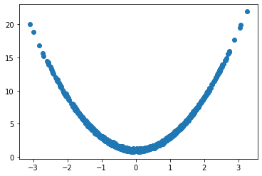
非线性关系数据集：y=x**2+1

# 设置随机数种子
torch.manual_seed(420)   

num_inputs = 2               # 两个特征
num_examples = 1000          # 总共一千条数据

# 线性方程系数
w_true = torch.tensor(2.)
b_true = torch.tensor(1.)

# 特征和标签取值
features = torch.randn(num_examples, num_inputs)
labels_true = torch.pow(features, 2) * w_true + b_true
labels = labels_true + torch.randn(size = labels_true.shape) * 0.1

# 可视化展示
plt.scatter(features, labels)

在这里插入图片描述

2、回归类数据集创建函数

为了方便后续使用，我们将上述过程封装在一个函数内。

# 回归类数据集创建函数
# 默认数据集：生成1000个样本，y=2*x1-x2+1，噪声项为0.01
def tensorGenReg(num_examples = 1000, w = [2, -1, 1], bias = True, delta = 0.01, deg = 1):
    """回归类数据集创建函数。

    :param num_examples: 创建数据集的数据量
    :param w: 包括截距的（如果存在）特征系数向量
    :param bias：是否需要截距
    :param delta：扰动项取值
    :param deg：方程次数
    :return: 生成的特征张和标签张量
    """
    
    if bias == True:
        num_inputs = len(w)-1                                                        # 特征张量
        features_true = torch.randn(num_examples, num_inputs)                        # 不包含全是1的列的特征张量
        w_true = torch.tensor(w[:-1]).reshape(-1, 1).float()                         # 自变量系数
        b_true = torch.tensor(w[-1]).float()                                         # 截距
        if num_inputs == 1:                                                          # 若输入特征只有1个，则不能使用矩阵乘法
            labels_true = torch.pow(features_true, deg) * w_true + b_true
        else:
            labels_true = torch.mm(torch.pow(features_true, deg), w_true) + b_true
        features = torch.cat((features_true, torch.ones(len(features_true), 1)), 1)  # 在特征张量的最后添加一列全是1的列
        labels = labels_true + torch.randn(size = labels_true.shape) * delta         
                
    else: 
        num_inputs = len(w)
        features = torch.randn(num_examples, num_inputs)
        w_true = torch.tensor(w).reshape(-1, 1).float()
        if num_inputs == 1:
            labels_true = torch.pow(features, deg) * w_true
        else:
            labels_true = torch.mm(torch.pow(features, deg), w_true)
        labels = labels_true + torch.randn(size = labels_true.shape) * delta
    return features, labels

注：上述函数无法创建带有交叉项的方程

测试函数性能

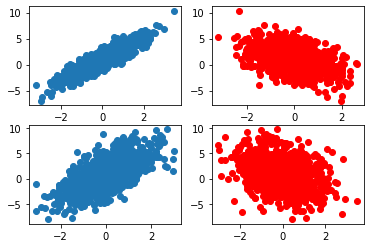
（1）线性关系，噪声项

# 生成1000个样本，y=2*x1-x2+1，噪声项为0.01
features, labels = tensorGenReg(num_examples = 1000, w = [2, -1, 1], bias = True, delta = 0.01, deg = 1)
# 生成1000个样本，y=2*x1-x2+1，噪声项为2
features2, labels2 = tensorGenReg(num_examples = 1000, w = [2, -1, 1], bias = True, delta = 2, deg = 1)

# 可视化展示
# 噪声项为0.01
plt.subplot(221)
plt.scatter(features[:, 0], labels)             # 第一个特征和标签的关系
plt.subplot(222)
plt.plot(features[:, 1], labels, 'ro')          # 第二个特征和标签的关系
# 噪声项为2
plt.subplot(223)
plt.scatter(features2[:, 0], labels2)             # 第一个特征和标签的关系
plt.subplot(224)
plt.plot(features2[:, 1], labels2, 'ro')          # 第二个特征和标签的关系

在这里插入图片描述
（2）二阶非线性关系

# 生成1000个样本，y=2*x1**2-x2**2+1，二阶非线性关系（两个特征）
features, labels = tensorGenReg(num_examples = 1000, w = [2, -1, 1], bias = True, delta = 0.01, deg = 2)
# 生成1000个样本，y= x1**2 ，二阶非线性关系（一个特征，无偏置b）
features3, labels3 = tensorGenReg(num_examples = 1000, w = [1], bias = False, delta = 0.01, deg = 2)

# 可视化展示
plt.subplot(221)
plt.scatter(features[:, 0], labels)             # 第一个特征x1和标签的关系
plt.subplot(222)
plt.plot(features[:, 1], labels, 'ro')          # 第二个特征x2和标签的关系
plt.subplot(223)
plt.plot(features3, labels3, 'yo')              # y= x1**2 关系

在这里插入图片描述

3、分类数据集手动创建方法

和回归模型的数据不同，分类模型数据的标签是离散值。

拥有两个特征的三分类的数据集

尝试创建一个拥有两个特征的三分类的数据集，每个类别包含500条数据，并且第一个类别的两个特征都服从均值为4、标准差为2的正态分布，第二个类别的两个特征都服从均值为-2、标准差为2的正态分布，第三个类别的两个特征都服从均值为-6、标准差为2的正态分布，创建过程如下:

# 设置随机数种子
torch.manual_seed(420)   

# 创建初始标记值
num_inputs = 2      # 特征数目
num_examples = 500  # 样本数目

# 创建自变量簇 x
data0 = torch.normal(4, 2, size=(num_examples, num_inputs))     # 类别1：Mean，Std(4,2)的正态分布
data1 = torch.normal(-2, 2, size=(num_examples, num_inputs))    # 类别2：Mean，Std(-2,2)的正态分布
data2 = torch.normal(-6, 2, size=(num_examples, num_inputs))    # 类别3：Mean，Std(-6,2)的正态分布

# 创建标签 y
label0 = torch.zeros(500)
label1 = torch.ones(500)
label2 = torch.full_like(label1, 2)

# 合并生成最终数据
features = torch.cat((data0, data1, data2)).float()
labels = torch.cat((label0, label1, label2)).long().reshape(-1, 1)  # 分类问题默认标签类型为整型

# 可视化展示
plt.scatter(features[:, 0], features[:, 1], c = labels)

在这里插入图片描述

4、分类数据集创建函数

同样，我们将上述创建分类函数的过程封装为一个函数。（均值，方差）变量可以控制数据整体离散程度，也就是后续建模分类的难以程度。如果每个分类数据集中心点较近（均值越小）、且每个类别的点内部方差较大（方差越大），则数据集整体离散程度较高（离散越高），反之离散程度较低。

# 分类数据集创建函数
# 默认数据集：特征2个，三分类，方差及均值为4,2，500样本。
def tensorGenCla(num_examples = 500, num_inputs = 2, num_class = 3, deg_dispersion = [4, 2], bias = False):
    """分类数据集创建函数。
    
    :param num_examples: 每个类别的数据数量
    :param num_inputs: 数据集特征数量
    :param num_class：数据集标签类别总数
    :param deg_dispersion：数据分布离散程度参数，需要输入一个列表，其中第一个参数表示每个类别数组均值的参考、第二个参数表示随机数组标准差。
    :param bias：建立模型逻辑回归模型时是否带入截距
    :return: 生成的特征张量和标签张量，其中特征张量是浮点型二维数组，标签张量是长正型二维数组。
    """
    
    cluster_l = torch.empty(num_examples, 1)                         # 每一类标签张量的形状
    mean_ = deg_dispersion[0]                                        # 每一类特征张量的均值的参考值
    std_ = deg_dispersion[1]                                         # 每一类特征张量的方差
    lf = []                                                          # 用于存储每一类特征张量的列表容器
    ll = []                                                          # 用于存储每一类标签张量的列表容器
    k = mean_ * (num_class-1) / 2                                    # 每一类特征张量均值的惩罚因子（视频中部分是+1，实际应该是-1）
    
    for i in range(num_class):
        data_temp = torch.normal(i*mean_-k, std_, size=(num_examples, num_inputs))     # 生成每一类张量
        lf.append(data_temp)                                                           # 将每一类张量添加到lf中
        labels_temp = torch.full_like(cluster_l, i)                                    # 生成类一类的标签
        ll.append(labels_temp)                                                         # 将每一类标签添加到ll中
        
    features = torch.cat(lf).float()
    labels = torch.cat(ll).long()
    
    if bias == True:
        features = torch.cat((features, torch.ones(len(features), 1)), 1)              # 在特征张量中添加一列全是1的列
    return features, labels

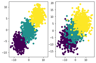
测试函数性能

# 设置随机数种子
torch.manual_seed(420)

# 创建数据
f, l = tensorGenCla(deg_dispersion = [6, 2])          # 离散程度较小
f1, l1 = tensorGenCla(deg_dispersion = [6, 4])        # 离散程度较大

# 绘制图像查看
plt.subplot(121)
plt.scatter(f[:, 0], f[:, 1], c = l)
plt.subplot(122)
plt.scatter(f1[:, 0], f1[:, 1], c = l1)

在这里插入图片描述

5、批量数据切分函数

在深度学习建模过程中，梯度下降是最常用的求解目标函数的优化方法，而针对不同类型、拥有不同函数特性的目标函数，所使用的梯度下降算法也各有不同。目前为止，我们判断 小批量梯度下降（MBGD） 是较为“普适”的优化算法，它既拥有随机梯度下降（SGD）的能够跨越局部最小值点的特性，同时又和批量梯度下降（BGD）一样，拥有相对较快的收敛速度（虽然速度略慢与BGD）。而在小批量梯度下降过程中，我们需要 对数据集进行分批量的切分，因此，在手动实现各类深度学习基础算法之前，我们需要定义数据集小批量切分的函数。

def data_iter(batch_size, features, labels):
    """
    数据切分函数
    
    :param batch_size: 每个子数据集包含多少数据
    :param featurs: 输入的特征张量
    :param labels：输入的标签张量
    :return sublist：包含batch_size个列表，每个列表切分后的特征和标签所组成 
    """

    num_examples = len(features)        # 样本数目
    indices = list(range(num_examples)) # 对应索引

    random.shuffle(indices)     # shuffle过程：将原序列乱序排列
    
    sublist = []
    for i in range(0, num_examples, batch_size):
        # 确保最后一组数据集的索引
        j = torch.tensor(indices[i: min(i + batch_size, num_examples)])
        # 按行选取第j行数据
        sublist.append([torch.index_select(features, 0, j), torch.index_select(labels, 0, j)])
    return sublist

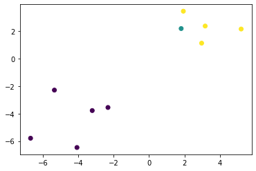
测试函数性能

# 设置随机数种子
torch.manual_seed(420)  

# 生成二分类数据集，特征2个，三分类，方差及均值为4,2，500样本。
features, labels = tensorGenCla(num_examples = 500, num_inputs = 2, num_class = 3, deg_dispersion = [4, 2], bias = False)  

# 数据集切分，每个数据集大小为10
l = data_iter(10, features, labels)

# 查看切分后的第一个数据集的
# 特征的第一个特征，特征的第二个特征和标签
plt.scatter(l[0][0][:, 0], l[0][0][:, 1], c = l[0][1])

在这里插入图片描述

6、Python中模块的编写与保存

将以下函数将保存到torchLearning.py文件中，即可在其他的py文件中调用方法函数。

tensorGenReg函数
tensorGenCla函数
data_iter函数

# 回归类数据集创建函数
# 默认数据集：生成1000个样本，y=2*x1-x2+1，噪声项为0.01
def tensorGenReg(num_examples = 1000, w = [2, -1, 1], bias = True, delta = 0.01, deg = 1):
    """回归类数据集创建函数。

    :param num_examples: 创建数据集的数据量
    :param w: 包括截距的（如果存在）特征系数向量
    :param bias：是否需要截距
    :param delta：扰动项取值
    :param deg：方程次数
    :return: 生成的特征张和标签张量
    """
    
    if bias == True:
        num_inputs = len(w)-1                                                        # 特征张量
        features_true = torch.randn(num_examples, num_inputs)                        # 不包含全是1的列的特征张量
        w_true = torch.tensor(w[:-1]).reshape(-1, 1).float()                         # 自变量系数
        b_true = torch.tensor(w[-1]).float()                                         # 截距
        if num_inputs == 1:                                                          # 若输入特征只有1个，则不能使用矩阵乘法
            labels_true = torch.pow(features_true, deg) * w_true + b_true
        else:
            labels_true = torch.mm(torch.pow(features_true, deg), w_true) + b_true
        features = torch.cat((features_true, torch.ones(len(features_true), 1)), 1)  # 在特征张量的最后添加一列全是1的列
        labels = labels_true + torch.randn(size = labels_true.shape) * delta         
                
    else: 
        num_inputs = len(w)
        features = torch.randn(num_examples, num_inputs)
        w_true = torch.tensor(w).reshape(-1, 1).float()
        if num_inputs == 1:
            labels_true = torch.pow(features, deg) * w_true
        else:
            labels_true = torch.mm(torch.pow(features, deg), w_true)
        labels = labels_true + torch.randn(size = labels_true.shape) * delta
    return features, labels

# 分类数据集创建函数
# 默认数据集：特征2个，三分类，方差及均值为4,2，500样本。
def tensorGenCla(num_examples = 500, num_inputs = 2, num_class = 3, deg_dispersion = [4, 2], bias = False):
    """分类数据集创建函数。
    
    :param num_examples: 每个类别的数据数量
    :param num_inputs: 数据集特征数量
    :param num_class：数据集标签类别总数
    :param deg_dispersion：数据分布离散程度参数，需要输入一个列表，其中第一个参数表示每个类别数组均值的参考、第二个参数表示随机数组标准差。
    :param bias：建立模型逻辑回归模型时是否带入截距
    :return: 生成的特征张量和标签张量，其中特征张量是浮点型二维数组，标签张量是长正型二维数组。
    """
    
    cluster_l = torch.empty(num_examples, 1)                         # 每一类标签张量的形状
    mean_ = deg_dispersion[0]                                        # 每一类特征张量的均值的参考值
    std_ = deg_dispersion[1]                                         # 每一类特征张量的方差
    lf = []                                                          # 用于存储每一类特征张量的列表容器
    ll = []                                                          # 用于存储每一类标签张量的列表容器
    k = mean_ * (num_class-1) / 2                                    # 每一类特征张量均值的惩罚因子（视频中部分是+1，实际应该是-1）
    
    for i in range(num_class):
        data_temp = torch.normal(i*mean_-k, std_, size=(num_examples, num_inputs))     # 生成每一类张量
        lf.append(data_temp)                                                           # 将每一类张量添加到lf中
        labels_temp = torch.full_like(cluster_l, i)                                    # 生成类一类的标签
        ll.append(labels_temp)                                                         # 将每一类标签添加到ll中
        
    features = torch.cat(lf).float()
    labels = torch.cat(ll).long()
    
    if bias == True:
        features = torch.cat((features, torch.ones(len(features), 1)), 1)              # 在特征张量中添加一列全是1的列
    return features, labels

# 批量数据切分函数
def data_iter(batch_size, features, labels):
    """
    数据切分函数
    
    :param batch_size: 每个子数据集包含多少数据
    :param featurs: 输入的特征张量
    :param labels：输入的标签张量
    :return l：包含batch_size个列表，每个列表切分后的特征和标签所组成 
    """
    num_examples = len(features)
    indices = list(range(num_examples))
    random.shuffle(indices)
    sublist = []
    for i in range(0, num_examples, batch_size):
        j = torch.tensor(indices[i: min(i + batch_size, num_examples)])
        sublist.append([torch.index_select(features, 0, j), torch.index_select(labels, 0, j)])
    return sublist

Lesson 12.3 线性回归建模实验

1、深度学习四步建模流程

在这里插入图片描述

2、线性回归的手动实现

# 1、数据集
torch.manual_seed(420)  
features, labels = tensorGenReg(num_examples=1000, w=[2, -1, 1], bias=True, delta=0.01, deg=1)

# 2、模型构建
def linreg(X,w): 
    return torch.mm(X, w)

# 3、损失函数 mse：误差平方和
def MSE_loss(yhat, y):
    total = y.numel()
    sse = torch.sum((yhat.reshape(-1, 1) - y.reshape(-1, 1)) ** 2) 
    return sse / total

# 4、优化算法 sgd：小批量梯度下降
def sgd(params, lr):
    params.data -= lr * params.grad         # (参数-学习率lr * 梯度)
    params.grad.zero_()

# 5、训练模型
# 初始化参数、参与训练的模型及函数、模型训练过程
def fit(batch_size=10, lr=0.03, num_epochs=3, w=torch.zeros(3, 1, requires_grad = True) ):
    '''训练模型函数
        batch_size: 每一个小批的数量
        lr: 学习率
        num_epochs: 训练过程遍历几次数据
        w: 随机设置初始权重
    '''
    
    # 参与训练的模型方程
    net = linreg           # 模型
    loss = MSE_loss        # 损失函数

    # 模型训练过程
    for epoch in range(num_epochs):
        for X, y in data_iter(batch_size, features, labels):
            l = loss(net(X, w), y)  
            l.backward()
            sgd(w, lr)
            
        train_l = loss(net(features, w), labels)
        print('epoch %d, loss %f' % (epoch + 1, train_l))

    return w    

fit()       # 返回训练好的参数

结果：

# 训练过程记录
epoch 1, loss 0.000128
epoch 2, loss 0.000102
epoch 3, loss 0.000102

# 训练好的参数
tensor([[ 1.9994],
        [-1.0004],
        [ 1.0009]], requires_grad=True)

3、线性回归的快速实现

# 定义核心参数
batch_size = 10      # 每一个小批的数量
lr = 0.03            # 学习率
num_epochs = 3       # 训练过程遍历几次数据

# 创建数据集
torch.manual_seed(420)   
features, labels = tensorGenReg(num_examples=1000, w=[2, -1, 1], bias=True, delta=0.01, deg=1)
features = features[:, :-1]       # 剔除最后全是1的列

# 数据封装加载
data = TensorDataset(features, labels)                                      
batchData = DataLoader(data, batch_size = batch_size, shuffle = True)       

# - Stage 1.定义模型
# - Stage 2.定义损失函数
# - Stage 3.定义优化方法
# - Stage 4.模型训练
class LR(nn.Module):
    def __init__(self, in_features=2, out_features=1):       # 定义模型的点线结构
        super(LR, self).__init__()
        self.linear = nn.Linear(in_features, out_features)
        
    def forward(self, x):                                    # 定义模型的正向传播规则
        out = self.linear(x)             
        return out
    
LR_model = LR()             # 模型
criterion = nn.MSELoss()    # 损失函数
optimizer = optim.SGD(LR_model.parameters(), lr = lr) # 优化方法


def fit(net, criterion, optimizer, batchdata, epochs):
    for epoch in range(epochs):
        for X, y in batchdata:
            yhat = net.forward(X)       # 向前传播
            loss = criterion(yhat, y)   # 计算损失函数
            optimizer.zero_grad()       # 清空梯度
            loss.backward()             # 反向传播
            optimizer.step()            # 更新梯度
        print('epoch %d, loss %f' % (epoch + 1, loss))

# 训练模型
fit(net = LR_model,         # 训练模型
    criterion = criterion,  # 损失函数
    optimizer = optimizer,  # 优化方法
    batchdata = batchData,  # 小批量数据
    epochs = num_epochs)    # 学习迭代次数
    
# 训练结果:(模型：LR，模型参数：w、b，损失函数值：MSE)
LR_model, list(LR_model.parameters()), criterion(LR_model(features), labels)

训练结果：

# 训练过程记录
epoch 1, loss 0.000259
epoch 2, loss 0.000087
epoch 3, loss 0.000156

# 训练好的模型
(LR(
   (linear): Linear(in_features=2, out_features=1, bias=True)
 ),
 [Parameter containing:
  tensor([[ 2.0004, -1.0000]], requires_grad=True),
  Parameter containing:
  tensor([1.0004], requires_grad=True)],
 tensor(0.0001, grad_fn=<MseLossBackward0>))

简单线性回归局限性
当自变量和因变量满足最高次方为2次方的多项式函数关系时，或者扰动项增加时，简单线性回归误差将迅速增大。
（1）自变量和因变量满足最高次方为2次方的多项式函数关系

#自变量和因变量满足最高次方为2次方的多项式函数关系

# 设置随机数种子
torch.manual_seed(420)   

# 创建数据集
features, labels = tensorGenReg(deg=2)
features = features[:, :-1]                                  # 剔除最后全是1的列

# 数据加载
data = TensorDataset(features, labels)
batchData = DataLoader(data, batch_size = batch_size, shuffle = True)

# 模型实例化
LR_model = LR()

# 定义优化算法
optimizer = optim.SGD(LR_model.parameters(), lr = 0.03)

# 模型训练
fit(net = LR_model, 
    criterion = criterion, 
    optimizer = optimizer, 
    batchdata = batchData, 
    epochs = num_epochs)

# MSE结果查看
criterion(LR_model(features), labels)

训练结果：

# 训练过程记录
epoch 1, loss 23.717789
epoch 2, loss 3.454563
epoch 3, loss 5.424092

# 训练好的模型的损失函数
tensor(10.1917, grad_fn=<MseLossBackward0>)

（2）增加扰动项

# 设置随机数种子
torch.manual_seed(420)   

# 创建数据集
features, labels = tensorGenReg(delta=2)
features = features[:, :-1]                                  # 剔除最后全是1的列

# 数据加载
data = TensorDataset(features, labels)
batchData = DataLoader(data, batch_size = batch_size, shuffle = True)

# 模型实例化
LR_model = LR()

# 定义优化算法
optimizer = optim.SGD(LR_model.parameters(), lr = 0.03)

# 模型训练
fit(net = LR_model, 
    criterion = criterion, 
    optimizer = optimizer, 
    batchdata = batchData, 
    epochs = num_epochs)

# MSE结果查看
criterion(LR_model(features), labels)

训练结果：

# 训练过程记录
epoch 1, loss 4.498693
epoch 2, loss 3.474763
epoch 3, loss 6.255614

# 训练好的模型的损失函数
tensor(4.0471, grad_fn=<MseLossBackward0>)

Lesson 12.4 逻辑回归建模实验

1. 逻辑回归手动实现

# 创建数据集
# def tensorGenCla(num_examples = 500, num_inputs = 2, num_class = 2, deg_dispersion = [4, 2], bias = True)
torch.manual_seed(420)   
features, labels = tensorGenCla(num_class=2, bias=True)

# 1、模型选择
# 2、损失函数
# 3、优化算法
# 4、训练模型

# 1、逻辑回归函数
def logistic(X,w): 
    z = torch.mm(X,w)
    zhat = 1/(1+torch.exp(-z))         # sigmoid
    return zhat     
# 2、损失函数
def cross_entropy(sigma, y):
    return(-(1/y.numel())*torch.sum((1-y)*torch.log(1-sigma)+y*torch.log(sigma)))
# 3、优化方法
def sgd(params, lr):
        params.data -= lr * params.grad 
        params.grad.zero_()

# 准确率函数
def accuracy(sigma, y):
    yhat = (sigma >= 0.5).float() 
    acc_bool = yhat.flatten() == y.flatten()
    acc = torch.mean(acc_bool.float())
    return(acc)

# 4、训练模型
# 初始化参数、参与训练的模型及函数、模型训练过程
def fit(batch_size=10, lr=0.03, num_epochs=3, w=torch.ones(3, 1, requires_grad = True) ):

    # 保存训练结果
    train_acc = []

    # 参与训练的模型方程
    net = logistic         # 模型：逻辑回归方程
    loss = cross_entropy   # 损失函数：交叉熵损失

    # 训练过程
    for epoch in range(num_epochs):
        for X, y in data_iter(batch_size, features, labels):
            l = loss(net(X, w), y)
            l.backward()
            sgd(w, lr)

        t_acc = accuracy(net(features, w), labels)
        train_l = loss(net(features, w), labels)
        print('epoch %d, loss %f, accuracy %f' % (epoch + 1, train_l, t_acc))
        train_acc.append(t_acc)

    return w,train_acc
    
# fit(batch_size=10, lr=0.03, num_epochs=3, w=torch.ones(3, 1, requires_grad = True) )
fit()

输出结果：

# 训练过程参数
epoch 1, loss 0.248594, accuracy 0.905000
epoch 2, loss 0.242073, accuracy 0.905000
epoch 3, loss 0.237481, accuracy 0.914000

# w
(tensor([[1.0035],
         [0.9764],
         [0.5778]], requires_grad=True),

# accuracy      
 [tensor(0.9050), tensor(0.9050), tensor(0.9140)])

模型调试

def fit_new(batch_size=10, lr=0.03, num_epochs=20, w=torch.ones(3, 1, requires_grad = True) ):

    # 保存训练结果
    train_acc = []

    # 参与训练的模型方程
    net = logistic         # 模型：逻辑回归方程
    loss = cross_entropy   # 损失函数：交叉熵损失

    # 执行迭代
    for i in range(num_epochs):
        for epoch in range(i):
            for X, y in data_iter(batch_size, features, labels):
                l = loss(net(X, w), y)
                l.backward()
                sgd(w, lr)
        train_acc.append(accuracy(net(features, w), labels))

    return train_acc

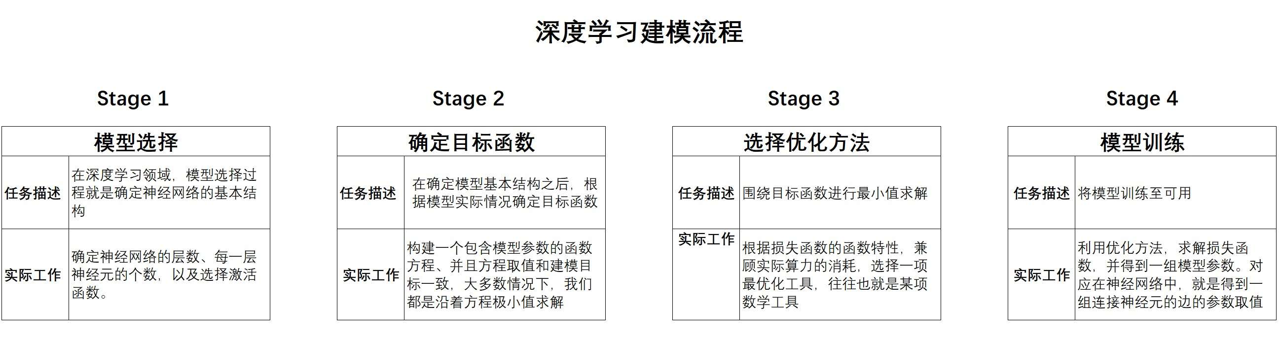
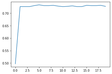
（1）学习次数增加
根据上述迭代三轮返回的准确率，能够看出整体还在增加，让我们再多迭代几轮查看结果

# 设置随机数种子
torch.manual_seed(420)   

# 迭代轮数为20
num_epochs=20
train_acc = fit_new(batch_size=10, lr=0.03, num_epochs=20, w=torch.ones(3, 1, requires_grad = True) )
    
# 绘制图像查看准确率变化情况
plt.plot(list(range(num_epochs)), train_acc)

在这里插入图片描述

能够看出，增加迭代次数之后，损失函数逼近最小值点，每次迭代梯度取值较小，整体准确率趋于平稳。
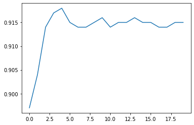
（2）增加数据复杂度

# 增加数据难度
features, labels = tensorGenCla(num_class=2, bias=True, deg_dispersion=[4, 4])

# 迭代轮数为20
num_epochs=20
train_acc = fit_new(batch_size=10, lr=0.03, num_epochs=20, w=torch.ones(3, 1, requires_grad = True) )
    
# 绘制图像查看准确率变化情况
plt.plot(list(range(num_epochs)), train_acc)

在这里插入图片描述

能够发现，随着数据情况变复杂，相同模型的准确率发生了很大的变化，下降许多。

2. 逻辑回归快速实现

batch_size = 10                                # 每一个小批的数量
lr = 0.03                                      # 学习率
num_epochs = 3                                 # 训练过程遍历几次数据

# 数据准备
# def tensorGenCla(num_examples = 500, num_inputs = 2, num_class = 2, deg_dispersion = [4, 2], bias = True)
torch.manual_seed(420)   
features, labels = tensorGenCla(num_class=2)
labels = labels.float()                                 # 损失函数要求标签也必须是浮点型

# 数据装载
data = TensorDataset(features, labels)            
batchData = DataLoader(data, batch_size = batch_size, shuffle = True)

# - Stage 1.定义模型
# - Stage 2.定义损失函数
# - Stage 3.定义优化方法
# - Stage 4.模型训练
class logisticR(nn.Module):
    def __init__(self, in_features=2, out_features=1):       # 定义模型的点线结构
        super(logisticR, self).__init__()
        self.linear = nn.Linear(in_features, out_features)
        
    def forward(self, x):                                    # 定义模型的正向传播规则
        out = self.linear(x)             
        return out

logic_model = logisticR()
criterion = nn.BCEWithLogitsLoss()
optimizer = optim.SGD(logic_model.parameters(), lr = lr)

def fit(net, criterion, optimizer, batchdata, epochs):

    # 创建列表容器
    train_acc = []
    
    for epoch in range(epochs):
        for X, y in batchdata:
            zhat = net.forward(X)
            loss = criterion(zhat, y)
            optimizer.zero_grad()
            loss.backward()
            optimizer.step()
            # print('epoch %d, loss %f' % (epoch + 1, loss)) 

# 模型准确率 
def acc_zhat(zhat, y):
    """输入为线性方程计算结果，输出为逻辑回归准确率的函数

    :param zhat：线性方程输出结果 
    :param y: 数据集标签张量
    :return：准确率 
    """
    sigma = 1/(1+torch.exp(-zhat))
    return accuracy(sigma, y)


# 训练模型
fit(net = logic_model,         # 训练模型
    criterion = criterion,  # 损失函数
    optimizer = optimizer,  # 优化方法
    batchdata = batchData,  # 小批量数据
    epochs = num_epochs)    # 学习迭代次数

# 模型训练结果
logic_model
# 查看模型参数
list(logic_model.parameters())
# 计算交叉熵损失
criterion(logic_model(features), labels)
# 计算函数准确率
acc_zhat(logic_model(features), labels)

输出结果：

# 模型训练结果
logisticR(
  (linear): Linear(in_features=2, out_features=1, bias=True)
)

# 查看模型参数
[Parameter containing:
 tensor([[0.8304, 0.8053]], requires_grad=True),
 Parameter containing:
 tensor([-0.2558], requires_grad=True)]

# 计算交叉熵损失
tensor(0.2293, grad_fn=<BinaryCrossEntropyWithLogitsBackward0>)

# 计算函数准确率
tensor(0.9130)

模型调试
（1）学习次数增加

torch.manual_seed(420)   

#创建数据
features, labels = tensorGenCla(num_class=2)                     
labels = labels.float()
                           
data = TensorDataset(features, labels)            
batchData = DataLoader(data, batch_size = batch_size, shuffle = True)

# 初始化核心参数
num_epochs = 20
LR1 = logisticR()
cr1 = nn.BCEWithLogitsLoss()
op1 = optim.SGD(LR1.parameters(), lr = lr)

# 创建列表容器
train_acc = []

# 执行建模
for epochs in range(num_epochs):
    fit(net = LR1, 
        criterion = cr1, 
        optimizer = op1, 
        batchdata = batchData, 
        epochs = epochs)
    epoch_acc = acc_zhat(LR1(features), labels)
    train_acc.append(epoch_acc)

# 绘制图像查看准确率变化情况
plt.plot(list(range(num_epochs)), train_acc)

在这里插入图片描述
（2）增加数据复杂度

torch.manual_seed(420)   

#创建数据
features, labels = tensorGenCla(num_class=2, deg_dispersion=[4, 4])                     
labels = labels.float()                           

# 数据封装与加载
data = TensorDataset(features, labels)            
batchData = DataLoader(data, batch_size = batch_size, shuffle = True)

# 初始化核心参数
num_epochs = 20
LR1 = logisticR()
cr1 = nn.BCEWithLogitsLoss()
op1 = optim.SGD(LR1.parameters(), lr = lr)

# 创建列表容器
train_acc = []

# 执行建模
for epochs in range(num_epochs):
    fit(net = LR1, 
        criterion = cr1, 
        optimizer = op1, 
        batchdata = batchData, 
        epochs = epochs)
    epoch_acc = acc_zhat(LR1(features), labels)
    train_acc.append(epoch_acc)

# 绘制图像查看准确率变化情况
plt.plot(list(range(num_epochs)), train_acc)

在这里插入图片描述

3. 模型调试入门

增加学习次数
增加数据复杂度

Lesson 12.5 softmax回归建模实验

1. softmax回归与max回归

我们都知道，softmax是用于挑选最大值的一种方法，通过以下公式对不同类的计算结果进行数值上的转化
$\delta_k = \frac{e^{z_k}}{\sum^Ke^k}$
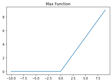
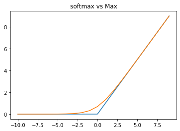
这种转化可以将结果放缩到0-1之间，并且使用softmax进行最大值的比较，相比max（softmax是max的柔化版本），能有效避免损失函数求解时在0点不可导的问题，损失函数的函数特性，将是后续我们选择优化算法的关键。具体我们可以通过下述图像进行比较。

from matplotlib import pyplot

def max_x(x, delta=0.):
    x = np.array(x)
    negative_idx = x < delta
    x[negative_idx] = 0.
    return x

x = np.array(range(-10, 10))
s_j = np.array(x)

hinge_loss = max_x(s_j, delta=1.)

pyplot.plot(s_j, hinge_loss)
pyplot.title("Max Function")

在这里插入图片描述

def cross_entropy_test(s_k, s_j):
    soft_max = 1/(1+np.exp(s_k - s_j))
    cross_entropy_loss = -np.log(soft_max)
    return cross_entropy_loss

s_i = 0
s_k = np.array(range(-10, 10))

soft_x = cross_entropy_test(s_k, s_i)

pyplot.plot(x, hinge_loss)
pyplot.plot(range(-10, 10), soft_x)
pyplot.title("softmax vs Max")

在这里插入图片描述

2. softmax回归手动实现

根据此前的介绍，面对分类问题，更为通用的处理办法将其转化为哑变量的形式，然后使用softmax回归进行处理，这种处理方式同样适用于二分类和多分类问题。此处以多分类问题为例，介绍softmax的手动实现形式。

# 设置随机数种子
torch.manual_seed(420)   

# 创建数据集
# tensorGenCla(num_examples = 500, num_inputs = 2, num_class = 3, deg_dispersion = [6, 2], bias = False):
features, labels = tensorGenCla(bias=True, deg_dispersion=[6, 2])

### 2.建模流程
# - Stage 1.模型选择
def softmax(X, w):
    m = torch.exp(torch.mm(X, w))
    sp = torch.sum(m, 1).reshape(-1, 1)
    return m / sp

# - Stage 2.确定目标函数
def m_cross_entropy(soft_z, y):
    y = y.long()
    prob_real = torch.gather(soft_z, 1, y)      # 批量索引
    return (-(1/y.numel()) * torch.log(prob_real).sum())

# - Stage 3.定义优化算法
def m_accuracy(soft_z, y):
    acc_bool = torch.argmax(soft_z, 1).flatten() == y.flatten()
    acc = torch.mean(acc_bool.float())
    return(acc)

def sgd(params, lr):
    params.data -= lr * params.grad 
    params.grad.zero_()

# - Stage.4 训练模型
def fit(batch_size=10, lr=0.03, num_epochs=3, w = torch.randn(3, 3, requires_grad = True)):

    # 参与训练的模型方程
    net = softmax                                     # 使用回归方程
    loss = m_cross_entropy                            # 交叉熵损失函数

    train_acc = []

    # 模型训练过程
    for epoch in range(num_epochs):
        for X, y in data_iter(batch_size, features, labels):
            l = loss(net(X, w), y)
            l.backward()
            sgd(w, lr)
        train_acc = m_accuracy(net(features, w), labels)
        print('epoch %d, acc %f' % (epoch + 1, train_acc))
    
    return w

fit()

# 训练过程参数
epoch 1, acc 0.889333
epoch 2, acc 0.944000
epoch 3, acc 0.957333

# w
tensor([[ 0.2785,  0.7989,  1.2963],
        [-0.4529,  0.0040,  0.5333],
        [-1.4873,  0.6896, -1.6629]], requires_grad=True)

模型调试

def fit_new(batch_size=10, lr=0.03, num_epochs=3, w = torch.randn(3, 3, requires_grad = True)):

    # 参与训练的模型方程
    net = softmax                                     # 使用回归方程
    loss = m_cross_entropy                            # 交叉熵损失函数

    train_acc = []

    # 模型训练过程
    for i in range(num_epochs):
        for epoch in range(i):
            for X, y in data_iter(batch_size, features, labels):
                l = loss(net(X, w), y)
                l.backward()
                sgd(w, lr)
        train_acc.append(m_accuracy(net(features, w), labels))
    
    return train_acc

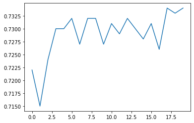
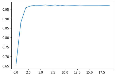
迭代次数

# 设置随机数种子
torch.manual_seed(420)   

# 迭代轮数
num_epochs = 20
train_acc = fit_new(batch_size=10, lr=0.03, num_epochs=20, w = torch.randn(3, 3, requires_grad = True))
    
# 绘制图像查看准确率变化情况
plt.plot(list(range(num_epochs)), train_acc)

在这里插入图片描述
在数据内部离散程度较低的情况下，模型收敛速度较快。

3. softmax回归快速实现

# - 定义核心参数
batch_size = 10                                # 每一个小批的数量
lr = 0.03                                      # 学习率
num_epochs = 3                                 # 训练过程遍历几次数据


# - 数据准备
# 设置随机数种子
torch.manual_seed(420)   

# 创建数据集
features, labels = tensorGenCla(deg_dispersion = [6, 2])
labels = labels.float()                           # 损失函数要求标签也必须是浮点型

# 数据加载
data = TensorDataset(features, labels)            
batchData = DataLoader(data, batch_size = batch_size, shuffle = True)

# - Stage 1.定义模型
# - Stage 2.定义损失函数
# - Stage 3.定义优化方法
# - Stage 4.模型训练
class softmaxR(nn.Module):
    def __init__(self, in_features=2, out_features=3, bias=False):       # 定义模型的点线结构
        super(softmaxR, self).__init__()
        self.linear = nn.Linear(in_features, out_features)
        
    def forward(self, x):                                    # 定义模型的正向传播规则
        out = self.linear(x)             
        return out

softmax_model = softmaxR()
criterion = nn.CrossEntropyLoss()
optimizer = optim.SGD(softmax_model.parameters(), lr = lr)

def fit(net, criterion, optimizer, batchdata, epochs):
    for epoch in range(epochs):
        for X, y in batchdata:
            zhat = net.forward(X)
            y = y.flatten().long()       # 损失函数计算要求转化为整数
            loss = criterion(zhat, y)
            optimizer.zero_grad()
            loss.backward()
            optimizer.step()

# 训练模型
fit(net = softmax_model,         # 训练模型
    criterion = criterion,  # 损失函数
    optimizer = optimizer,  # 优化方法
    batchdata = batchData,  # 小批量数据
    epochs = num_epochs)    # 学习迭代次数

# 查看模型训练结果
softmax_model
# 查看模型参数
print(list(softmax_model.parameters()))
# 计算交叉熵损失
criterion(softmax_model(features), labels.flatten().long())
# 借助F.softmax函数，计算准确率
m_accuracy(F.softmax(softmax_model(features), 1), labels)

# 查看模型训练结果
softmaxR(
  (linear): Linear(in_features=2, out_features=3, bias=True)
)
# 查看模型参数w,b
[Parameter containing:
tensor([[-0.9974, -0.6224],
        [-0.5061, -0.2205],
        [-0.0265,  0.2932]], requires_grad=True), Parameter containing:
tensor([-0.8604,  1.1235, -1.3058], requires_grad=True)]

# 计算交叉熵损失
tensor(0.1799, grad_fn=<NllLossBackward0>)

# 借助F.softmax函数，计算准确率
tensor(0.9573)

模型调试
（1）学习迭代次数

# 设置随机数种子
torch.manual_seed(420)   

# 创建数据集
features, labels = tensorGenCla(deg_dispersion = [6, 2])
labels = labels.float()                           # 损失函数要求标签也必须是浮点型

data = TensorDataset(features, labels)            
batchData = DataLoader(data, batch_size = batch_size, shuffle = True)

# 初始化核心参数
num_epochs = 20
SF1 = softmaxR()
cr1 = nn.CrossEntropyLoss()
op1 = optim.SGD(SF1.parameters(), lr = lr)

# 创建列表容器
train_acc = []

# 执行建模
for epochs in range(num_epochs):
    fit(net = SF1, 
        criterion = cr1, 
        optimizer = op1, 
        batchdata = batchData, 
        epochs = epochs)
    epoch_acc = m_accuracy(F.softmax(SF1(features), 1), labels)
    train_acc.append(epoch_acc)

# 绘制图像查看准确率变化情况
plt.plot(list(range(num_epochs)), train_acc)

在这里插入图片描述
和手动实现相同，此处模型也展示了非常快的收敛速度。当然需要再次强调，当num_epochs=20时，SF1参数已经训练了(19+18+…+1)次了。

（2）数据集难度

# 设置随机数种子
torch.manual_seed(420)   

# 创建数据集
features, labels = tensorGenCla(deg_dispersion = [6, 4])
labels = labels.float()                           # 损失函数要求标签也必须是浮点型

data = TensorDataset(features, labels)            
batchData = DataLoader(data, batch_size = batch_size, shuffle = True)

# 初始化核心参数
num_epochs = 20
SF1 = softmaxR()
cr1 = nn.CrossEntropyLoss()
op1 = optim.SGD(SF1.parameters(), lr = lr)

# 创建列表容器
train_acc = []

# 执行建模
for epochs in range(num_epochs):
    fit(net = SF1, 
        criterion = cr1, 
        optimizer = op1, 
        batchdata = batchData, 
        epochs = epochs)
    epoch_acc = m_accuracy(F.softmax(SF1(features), 1), labels)
    train_acc.append(epoch_acc)

# 绘制图像查看准确率变化情况
plt.plot(list(range(num_epochs)), train_acc)

在这里插入图片描述
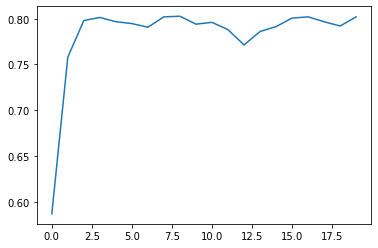
我们发现，收敛速度仍然很快，模型很快就到达了比较稳定的状态。但和此前的逻辑回归实验相同，模型结果虽然比较稳定，但受到数据集分类难度提升影响，模型准确率却不高，基本维持在80%左右。一般来说，此时就代表模型抵达了判别效力上界，此时模型已经无法有效捕捉数据集中规律。

模型判别效力上界
但到底什么叫做模型判别效力上界呢？从根本上来说就是模型已经到达（逼近）损失函数的最小值点，但模型的评估指标却无法继续提升。首先，我们可以初始选择多个w来观察损失函数是否已经逼近最小值点而不是落在了局部最小值点附近。

# 初始化核心参数
cr1 = nn.CrossEntropyLoss()

# 创建列表容器
train_acc = []

# 执行建模
for i in range(10):
    SF1 = softmaxR()
    op1 = optim.SGD(SF1.parameters(), lr = lr)
    fit(net = SF1, 
        criterion = cr1, 
        optimizer = op1, 
        batchdata = batchData, 
        epochs = 10)
    epoch_acc = m_accuracy(F.softmax(SF1(features), 1), labels)
    train_acc.append(epoch_acc)
train_acc

初始化不同的w发现最终模型准确率仍然是80%左右，也从侧面印证迭代过程没有问题，模型已经到达（逼近）最小值点。也就是说问题并不是出在损失函数的求解上，而是出在损失函数的构造上。此时的损失函数哪怕取得最小值点，也无法进一步提升模型效果。而损失函数的构造和模型的构造直接相关，此时若要进一步提升模型效果，就需要调整模型结构了。这也将是下一阶段模型调优核心讨论的内容。

白白白飘

关注

19
点赞
踩
8

收藏

觉得还不错? 一键收藏
打赏
1
评论
pytorch-12 深度学习基础网络的数据集创建及手动搭建实现

尽管深度学习也属于机器学习范畴，基本的建模理念和机器学习类似，比如需要确定目标函数和损失函数、找到合适的优化算法对参数进行求解等等，但利用PyTorch在进行建模的过程却和和最大的机器学习库Scikit-Learn中定义的机器学习建模方法有较大的差别。那为何PyTorch的整个实现过程看似会更加复杂？归根结底，还是和深度学习建模的特殊性有关。
复制链接

扫一扫