STGCN_IJCAI-18-master代码解读（五）：layers.py

解读layers.py

import tensorflow._api.v2.compat.v1 as tf
tf.disable_v2_behavior()

gconv（）函数

def gconv(x, theta, Ks, c_in, c_out):
    '''
    Spectral-based graph convolution function.
    :param x: tensor, [batch_size, n_route, c_in].
    :param theta: tensor, [Ks*c_in, c_out], trainable kernel parameters.
    :param Ks: int, kernel size of graph convolution.
    :param c_in: int, size of input channel.
    :param c_out: int, size of output channel.
    :return: tensor, [batch_size, n_route, c_out].
    '''
    # graph kernel: tensor, [n_route, Ks*n_route]
    kernel = tf.get_collection('graph_kernel')[0]
    n = tf.shape(kernel)[0]
    # x -> [batch_size, c_in, n_route] -> [batch_size*c_in, n_route]
    x_tmp = tf.reshape(tf.transpose(x, [0, 2, 1]), [-1, n])
    # x_mul = x_tmp * ker -> [batch_size*c_in, Ks*n_route] -> [batch_size, c_in, Ks, n_route]
    x_mul = tf.reshape(tf.matmul(x_tmp, kernel), [-1, c_in, Ks, n])
    # x_ker -> [batch_size, n_route, c_in, K_s] -> [batch_size*n_route, c_in*Ks]
    x_ker = tf.reshape(tf.transpose(x_mul, [0, 3, 1, 2]), [-1, c_in * Ks])
    # x_gconv -> [batch_size*n_route, c_out] -> [batch_size, n_route, c_out]
    x_gconv = tf.reshape(tf.matmul(x_ker, theta), [-1, n, c_out])
    return x_gconv

这个函数实现了基于频谱的图卷积（Spectral-based Graph Convolution）。图卷积是一种在图结构数据上进行的卷积操作。基于频谱的方法通常使用图的拉普拉斯矩阵的特征分解来定义卷积。

参数解释：

• x: 输入张量，形状为[batch_size, n_route, c_in]，其中batch_size是批大小，n_route是图中节点的数量，c_in是输入通道的数量。
• theta: 训练可的卷积核参数，形状为[Ks * c_in, c_out]。
• Ks: 图卷积的核大小。
• c_in: 输入通道的大小。
• c_out: 输出通道的大小。

过程解释：

1. 获取图核（Kernel）: 使用tf.get_collection('graph_kernel')[0]从TensorFlow的集合中获取预先计算的图核。

2. 调整输入张量形状:

   • 使用tf.transpose和tf.reshape重新排列和改变x的形状，以便进行矩阵乘法。

3. 应用图核:

   • 通过矩阵乘法tf.matmul将输入x与图核相乘。
   • 再次调整形状和转置以适应图卷积。

4. 执行图卷积操作:

   • 使用tf.matmul将调整后的输入与训练参数theta进行矩阵乘法。
   • 通过tf.reshape将输出调整回 [batch_size, n_route, c_out] 的形状。

最后，函数返回图卷积的输出，该输出是一个形状为[batch_size, n_route, c_out]的张量。

这种基于频谱的图卷积通常用于处理具有复杂结构和相互依赖性的数据，例如社交网络、通信网络或交通网络。这样的卷积能够捕捉到图结构中的高级依赖关系。

layer_norm（）函数

def layer_norm(x, scope):
    '''
    Layer normalization function.
    :param x: tensor, [batch_size, time_step, n_route, channel].
    :param scope: str, variable scope.
    :return: tensor, [batch_size, time_step, n_route, channel].
    '''
    _, _, N, C = x.get_shape().as_list()
    mu, sigma = tf.nn.moments(x, axes=[2, 3], keep_dims=True)

    with tf.variable_scope(scope):
        gamma = tf.get_variable('gamma', initializer=tf.ones([1, 1, N, C]))
        beta = tf.get_variable('beta', initializer=tf.zeros([1, 1, N, C]))
        _x = (x - mu) / tf.sqrt(sigma + 1e-6) * gamma + beta
    return _x

这个函数实现了层归一化（Layer Normalization），这是一种在神经网络中常用的归一化技术。层归一化主要用于稳定神经网络的训练。

参数解释：

• x: 输入张量，其形状是 [batch_size, time_step, n_route, channel]。其中 batch_size 是批量大小，time_step 是时间步长，n_route 是图（或空间）中的节点数，channel 是输入通道数。
• scope: 变量作用域的名字，用于在 TensorFlow 中唯一标识一组变量。

过程解释：

1. 计算均值和方差: 使用 tf.nn.moments 计算输入张量 x 沿着第2和第3维（也就是 n_route 和 channel 维度）的均值（mu）和方差（sigma）。keep_dims=True 保持输出的维度与输入一致，方便后续的广播操作。

2. 定义可训练参数: 在给定的作用域 scope 下，

   • gamma 是一个可训练的缩放参数，初始化为 1。
   • beta 是一个可训练的偏移参数，初始化为 0。
     这两个参数都有与输入相同的空间和通道维度 [1, 1, N, C]。

3. 应用层归一化:

   • 从输入 x 中减去均值 mu，然后除以 sqrt(sigma + 1e-6) 来归一化。
   • 使用 gamma 和 beta 进行缩放和偏移。
     这里加入一个小常数 1e-6 是为了数值稳定性，防止除以0。

函数返回经过层归一化处理后的张量 _x，其形状与输入 x 相同。

总体而言，这个函数的目的是使得网络中每一层的输出有更加稳定的分布，从而有助于网络的训练。

temporal_conv_layer（）函数

def temporal_conv_layer(x, Kt, c_in, c_out, act_func='relu'):
    '''
    Temporal convolution layer.
    :param x: tensor, [batch_size, time_step, n_route, c_in].
    :param Kt: int, kernel size of temporal convolution.
    :param c_in: int, size of input channel.
    :param c_out: int, size of output channel.
    :param act_func: str, activation function.
    :return: tensor, [batch_size, time_step-Kt+1, n_route, c_out].
    '''
    _, T, n, _ = x.get_shape().as_list()

    if c_in > c_out:
        w_input = tf.get_variable('wt_input', shape=[1, 1, c_in, c_out], dtype=tf.float32)
        tf.add_to_collection(name='weight_decay', value=tf.nn.l2_loss(w_input))
        x_input = tf.nn.conv2d(x, w_input, strides=[1, 1, 1, 1], padding='SAME')
    elif c_in < c_out:
        # if the size of input channel is less than the output,
        # padding x to the same size of output channel.
        # Note, _.get_shape() cannot convert a partially known TensorShape to a Tensor.
        x_input = tf.concat([x, tf.zeros([tf.shape(x)[0], T, n, c_out - c_in])], axis=3)
    else:
        x_input = x

    # keep the original input for residual connection.
    x_input = x_input[:, Kt - 1:T, :, :]

    if act_func == 'GLU':
        # gated liner unit
        wt = tf.get_variable(name='wt', shape=[Kt, 1, c_in, 2 * c_out], dtype=tf.float32)
        tf.add_to_collection(name='weight_decay', value=tf.nn.l2_loss(wt))
        bt = tf.get_variable(name='bt', initializer=tf.zeros([2 * c_out]), dtype=tf.float32)
        x_conv = tf.nn.conv2d(x, wt, strides=[1, 1, 1, 1], padding='VALID') + bt
        return (x_conv[:, :, :, 0:c_out] + x_input) * tf.nn.sigmoid(x_conv[:, :, :, -c_out:])
    else:
        wt = tf.get_variable(name='wt', shape=[Kt, 1, c_in, c_out], dtype=tf.float32)
        tf.add_to_collection(name='weight_decay', value=tf.nn.l2_loss(wt))
        bt = tf.get_variable(name='bt', initializer=tf.zeros([c_out]), dtype=tf.float32)
        x_conv = tf.nn.conv2d(x, wt, strides=[1, 1, 1, 1], padding='VALID') + bt
        if act_func == 'linear':
            return x_conv
        elif act_func == 'sigmoid':
            return tf.nn.sigmoid(x_conv)
        elif act_func == 'relu':
            return tf.nn.relu(x_conv + x_input)
        else:
            raise ValueError(f'ERROR: activation function "{act_func}" is not defined.')

这个函数实现了一个时间卷积层（Temporal Convolution Layer），这是一种在序列数据上应用的卷积层。

参数解释：

• x: 输入张量，其形状是 [batch_size, time_step, n_route, c_in]。其中 batch_size 是批量大小，time_step 是时间步长，n_route 是图（或空间）中的节点数，c_in 是输入通道数。
• Kt: 时间卷积核的大小。
• c_in: 输入通道的数量。
• c_out: 输出通道的数量。
• act_func: 激活函数的类型。它可以是 ‘relu’、‘sigmoid’、‘linear’ 或 ‘GLU’（门控线性单元）。

过程解释：

1. 调整输入通道数：如果输入通道数 c_in 和输出通道数 c_out 不相等，那么将通过卷积或填充来使它们相等。

2. 保留残差连接的输入：x_input 存储了原始输入的一个子集，这个子集将用于残差连接。

3. 应用时间卷积：

   • 如果激活函数是 ‘GLU’（门控线性单元），它将执行一个特定的门控操作。
   • 否则，它将应用一个标准的卷积操作。

4. 应用激活函数：根据 act_func 参数应用相应的激活函数。

5. 添加权重衰减：通过将权重的 L2 范数添加到名为 ‘weight_decay’ 的集合中，实现权重衰减。

返回的是一个形状为 [batch_size, time_step-Kt+1, n_route, c_out] 的张量，这个张量是经过时间卷积和激活函数处理后的结果。

这个函数可以用于时空图网络中，特别是当我们需要在时间维度上应用卷积操作时。

spatio_conv_layer（）函数

def spatio_conv_layer(x, Ks, c_in, c_out):
    '''
    Spatial graph convolution layer.
    :param x: tensor, [batch_size, time_step, n_route, c_in].
    :param Ks: int, kernel size of spatial convolution.
    :param c_in: int, size of input channel.
    :param c_out: int, size of output channel.
    :return: tensor, [batch_size, time_step, n_route, c_out].
    '''
    _, T, n, _ = x.get_shape().as_list()

    if c_in > c_out:
        # bottleneck down-sampling
        w_input = tf.get_variable('ws_input', shape=[1, 1, c_in, c_out], dtype=tf.float32)
        tf.add_to_collection(name='weight_decay', value=tf.nn.l2_loss(w_input))
        x_input = tf.nn.conv2d(x, w_input, strides=[1, 1, 1, 1], padding='SAME')
    elif c_in < c_out:
        # if the size of input channel is less than the output,
        # padding x to the same size of output channel.
        # Note, _.get_shape() cannot convert a partially known TensorShape to a Tensor.
        x_input = tf.concat([x, tf.zeros([tf.shape(x)[0], T, n, c_out - c_in])], axis=3)
    else:
        x_input = x

    ws = tf.get_variable(name='ws', shape=[Ks * c_in, c_out], dtype=tf.float32)
    tf.add_to_collection(name='weight_decay', value=tf.nn.l2_loss(ws))
    variable_summaries(ws, 'theta')
    bs = tf.get_variable(name='bs', initializer=tf.zeros([c_out]), dtype=tf.float32)
    # x -> [batch_size*time_step, n_route, c_in] -> [batch_size*time_step, n_route, c_out]
    x_gconv = gconv(tf.reshape(x, [-1, n, c_in]), ws, Ks, c_in, c_out) + bs
    # x_g -> [batch_size, time_step, n_route, c_out]
    x_gc = tf.reshape(x_gconv, [-1, T, n, c_out])
    return tf.nn.relu(x_gc[:, :, :, 0:c_out] + x_input)

这个函数实现了一个空间图卷积层（Spatial Graph Convolution Layer），这是一种在图结构数据上应用的卷积层。

参数解释：

• x: 输入张量，其形状是 [batch_size, time_step, n_route, c_in]。其中 batch_size 是批量大小，time_step 是时间步长，n_route 是图（或空间）中的节点数，c_in 是输入通道数。
• Ks: 空间卷积核的大小。
• c_in: 输入通道的数量。
• c_out: 输出通道的数量。

过程解释：

1. 调整输入通道数：如果输入通道数 c_in 和输出通道数 c_out 不相等，那么通过卷积或填充调整 x 使它们匹配。

2. 初始化权重和偏置项：

   • ws: 空间卷积的权重矩阵。
   • bs: 偏置向量。

3. 执行图卷积：使用 gconv 函数（该函数需要在上下文中定义）来进行图卷积操作。gconv 函数应用了空间卷积，它取形状为 [batch_size*time_step, n_route, c_in] 的张量作为输入，并返回形状为 [batch_size*time_step, n_route, c_out] 的张量。

4. 添加偏置并激活：在图卷积后，加上偏置项 bs，然后应用ReLU激活函数。

5. 残差连接：图卷积的输出与原始输入（可能已经调整过通道数）相加。这是一种简单的残差连接。

6. 添加权重衰减：通过将权重的L2损失添加到名为 ‘weight_decay’ 的集合中，实现权重衰减。

最后，函数返回一个形状为 [batch_size, time_step, n_route, c_out] 的张量。

这个空间图卷积层通常用于处理图结构的数据，尤其是在时空网络（ST-Net）中，这些网络同时考虑时间和空间维度。

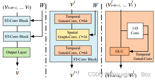
st_conv_block（）函数

def st_conv_block(x, Ks, Kt, channels, scope, keep_prob, act_func='GLU'):
    '''
    Spatio-temporal convolutional block, which contains two temporal gated convolution layers
    and one spatial graph convolution layer in the middle.
    :param x: tensor, batch_size, time_step, n_route, c_in].
    :param Ks: int, kernel size of spatial convolution.
    :param Kt: int, kernel size of temporal convolution.
    :param channels: list, channel configs of a single st_conv block.
    :param scope: str, variable scope.
    :param keep_prob: placeholder, prob of dropout.
    :param act_func: str, activation function.
    :return: tensor, [batch_size, time_step, n_route, c_out].
    '''
    c_si, c_t, c_oo = channels

    with tf.variable_scope(f'stn_block_{scope}_in'):
        x_s = temporal_conv_layer(x, Kt, c_si, c_t, act_func=act_func)
        x_t = spatio_conv_layer(x_s, Ks, c_t, c_t)
    with tf.variable_scope(f'stn_block_{scope}_out'):
        x_o = temporal_conv_layer(x_t, Kt, c_t, c_oo)
    x_ln = layer_norm(x_o, f'layer_norm_{scope}')
    return tf.nn.dropout(x_ln, keep_prob)

这个函数实现了一个时空卷积块（Spatio-Temporal Convolutional Block），通常用于处理同时具有时间和空间结构的数据。例如，在交通流预测或视频分析中，这种类型的网络结构可能特别有用。

参数解释：

• x: 输入张量，形状为 [batch_size, time_step, n_route, c_in]。

  • batch_size: 批次大小。
  • time_step: 时间步长。
  • n_route: 路由（或节点）数量。
  • c_in: 输入通道数量。

• Ks: 空间卷积核大小。

• Kt: 时间卷积核大小。

• channels: 一个包含三个元素的列表，分别表示输入、中间和输出通道的数量。

  • c_si: 输入通道数量。
  • c_t: 中间（或临时）通道数量。
  • c_oo: 输出通道数量。

• scope: 变量作用域的名称。

• keep_prob: Dropout 的保留概率。

• act_func: 激活函数类型（如 ‘GLU’）。

过程解释：

1. 时间卷积层（Temporal Convolution Layer）: 使用 temporal_conv_layer 函数对输入 x 进行时间卷积，输出通道数量是 c_t。

2. 空间卷积层（Spatial Convolution Layer）: 使用 spatio_conv_layer 函数对上一步的输出进行空间卷积。输入和输出通道数都是 c_t。

3. 时间卷积层（Temporal Convolution Layer）: 使用 temporal_conv_layer 函数对上一步的输出进行第二次时间卷积。输出通道数量是 c_oo。

4. 层归一化（Layer Normalization）: 使用 layer_norm 函数对上一步的输出进行层归一化。

5. Dropout: 使用 Dropout 对归一化后的输出进行正则化。

函数最后返回一个形状为 [batch_size, time_step, n_route, c_out] 的张量。

这个时空卷积块结合了时间和空间的信息，通过两个时间卷积层和一个空间卷积层来实现这一目标。层归一化和 Dropout 进一步帮助网络训练和泛化。

fully_con_layer（）函数

def fully_con_layer(x, n, channel, scope):
    '''
    Fully connected layer: maps multi-channels to one.
    :param x: tensor, [batch_size, 1, n_route, channel].
    :param n: int, number of route / size of graph.
    :param channel: channel size of input x.
    :param scope: str, variable scope.
    :return: tensor, [batch_size, 1, n_route, 1].
    '''
    w = tf.get_variable(name=f'w_{scope}', shape=[1, 1, channel, 1], dtype=tf.float32)
    tf.add_to_collection(name='weight_decay', value=tf.nn.l2_loss(w))
    b = tf.get_variable(name=f'b_{scope}', initializer=tf.zeros([n, 1]), dtype=tf.float32)
    return tf.nn.conv2d(x, w, strides=[1, 1, 1, 1], padding='SAME') + b

这个函数实现了一个全连接层（Fully Connected Layer），但它使用卷积操作来达到相同的效果。全连接层将多个输入通道映射到单一输出通道，通常用于最后的预测或分类任务。

参数解释：

• x: 输入张量，其形状为 [batch_size, 1, n_route, channel]。

  • batch_size: 批处理的大小。
  • 1: 这通常是时间或空间维度，但在这里设置为1。
  • n_route: 路由（或节点）的数量。
  • channel: 输入的通道数。

• n: 整数，表示路由（或图的大小）的数量。

• channel: 输入张量 x 的通道大小。

• scope: 变量的作用域名称。

过程解释：

1. 权重初始化：权重 w 的形状是 [1, 1, channel, 1]，初始化为浮点数类型。权重用于卷积操作。

2. 偏置初始化：偏置 b 的形状是 [n, 1]，初始化为全零。偏置用于卷积操作后的加法。

3. 卷积操作：使用输入 x 和权重 w 进行卷积操作。步长（strides）是 [1, 1, 1, 1]，填充（padding）是 'SAME'，意味着输出的空间尺寸与输入相同。

4. 加偏置：将卷积结果与偏置 b 相加。

函数最后返回一个形状为 [batch_size, 1, n_route, 1] 的张量。

总体而言，这个全连接层通过卷积操作将每个路由（或节点）的多个特征通道减少到一个单一的输出通道。这样做通常用于减少模型的复杂性和进行预测或分类。

output_layer（）函数

def output_layer(x, T, scope, act_func='GLU'):
    '''
    Output layer: temporal convolution layers attach with one fully connected layer,
    which map outputs of the last st_conv block to a single-step prediction.
    :param x: tensor, [batch_size, time_step, n_route, channel].
    :param T: int, kernel size of temporal convolution.
    :param scope: str, variable scope.
    :param act_func: str, activation function.
    :return: tensor, [batch_size, 1, n_route, 1].
    '''
    _, _, n, channel = x.get_shape().as_list()

    # maps multi-steps to one.
    with tf.variable_scope(f'{scope}_in'):
        x_i = temporal_conv_layer(x, T, channel, channel, act_func=act_func)
    x_ln = layer_norm(x_i, f'layer_norm_{scope}')
    with tf.variable_scope(f'{scope}_out'):
        x_o = temporal_conv_layer(x_ln, 1, channel, channel, act_func='sigmoid')
    # maps multi-channels to one.
    x_fc = fully_con_layer(x_o, n, channel, scope)
    return x_fc

这个函数实现了模型的输出层，该层是预测或分类任务的最后一步。该函数使用两个时间卷积层（temporal convolution layers）和一个全连接层（fully connected layer）来将多步和多通道的输入映射到单步和单通道的输出。

参数解释：

• x: 输入张量，其形状为 [batch_size, time_step, n_route, channel]。

  • batch_size: 批处理的大小。
  • time_step: 时间步长。
  • n_route: 路由（或节点）的数量。
  • channel: 输入的通道数。

• T: 整数，时间卷积的内核大小（kernel size）。

• scope: 变量的作用域名称。

• act_func: 激活函数，这里默认是 ‘GLU’（门控线性单元）。

过程解释：

1. 第一个时间卷积层: 在作用域 {scope}_in 下，通过调用 temporal_conv_layer 函数来应用第一个时间卷积层。这里用相同的通道数作为输入和输出，并使用用户定义的激活函数（默认是 ‘GLU’）。

2. 层标准化（Layer Normalization）: 使用 layer_norm 函数进行层标准化，以加速训练并提高模型性能。

3. 第二个时间卷积层: 在作用域 {scope}_out 下，使用内核大小为 1 的时间卷积层，激活函数是 ‘sigmoid’。

4. 全连接层: 通过调用 fully_con_layer 函数，将多通道输入映射到单一输出通道。这通常用于最后的预测或分类任务。

最后，该函数返回一个形状为 [batch_size, 1, n_route, 1] 的输出张量。

总体来说，output_layer 函数将多步长和多通道的输入通过一系列时间卷积和一个全连接层映射到一个单步和单通道的输出，这通常用于时间序列预测或分类任务。

variable_summaries（）函数

def variable_summaries(var, v_name):
    '''
    Attach summaries to a Tensor (for TensorBoard visualization).
    Ref: https://zhuanlan.zhihu.com/p/33178205
    :param var: tf.Variable().
    :param v_name: str, name of the variable.
    '''
    with tf.name_scope('summaries'):
        mean = tf.reduce_mean(var)
        tf.summary.scalar(f'mean_{v_name}', mean)

        with tf.name_scope(f'stddev_{v_name}'):
            stddev = tf.sqrt(tf.reduce_mean(tf.square(var - mean)))
        tf.summary.scalar(f'stddev_{v_name}', stddev)

        tf.summary.scalar(f'max_{v_name}', tf.reduce_max(var))
        tf.summary.scalar(f'min_{v_name}', tf.reduce_min(var))

        tf.summary.histogram(f'histogram_{v_name}', var)

这个函数旨在为给定的 TensorFlow 变量生成和附加一系列的统计摘要，这些摘要可以用于 TensorBoard 可视化。通过 TensorBoard，您可以更加直观地理解、调试和优化 TensorFlow 程序。

参数解释：

• var: 这是一个 TensorFlow 变量，它是我们要生成统计数据的目标。
• v_name: 这是一个字符串，表示变量的名称，用于在 TensorBoard 上标识和组织相关的摘要信息。

函数实现说明：

1. 定义摘要的名称作用域: with tf.name_scope('summaries'): 定义了摘要统计的顶级名称作用域。名称作用域在 TensorBoard 中提供了组织结构。

2. 计算平均值: 使用 tf.reduce_mean 函数计算变量的平均值，并创建一个摘要标量记录平均值。

3. 计算标准差: 首先，计算变量与其均值的差的平方的均值，然后计算其平方根以得到标准差。

4. 记录最大值和最小值: 使用 tf.reduce_max 和 tf.reduce_min 函数分别计算变量的最大值和最小值，并为每个值创建一个摘要标量。

5. 生成直方图: 使用 tf.summary.histogram 为变量创建一个直方图摘要。这在 TensorBoard 中可视化时，可以看到变量值分布的变化。

总体而言，此函数为指定的 TensorFlow 变量生成了一系列有关其统计信息的摘要，并且可以在 TensorBoard 中可视化这些摘要。这对于理解模型中变量的行为、分布和其他统计特性非常有用。