用python动手学统计学_3-6正态分布

正态分布

概率密度

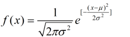
实现以均值为4、方差为0.64，随机变量为3计算概率密度：

# 用于数值计算的库
import numpy as np
import pandas as pd
import scipy as sp
from scipy import stats

# 用于绘图的库
from matplotlib import pyplot as plt
import seaborn as sns
sns.set()

# 设置浮点数打印精度
%precision 3
# 在 Jupyter Notebook 里显示图形
%matplotlib inline

# 均值为 4 标准差为 0.8 的正态分布在随机变量为 3 时的概率密度
x = 3
mu = 4
sigma = 0.8

1 / (sp.sqrt(2 * sp.pi * sigma**2)) * \
    sp.exp(- ((x - mu)**2) / (2 * sigma**2))
#0.22831135673627742

也可以使用scipy.stats.norm.pdf()函数

stats.norm.pdf(loc = 4, scale = 0.8, x = 3)
#0.228

norm_dist = stats.norm(loc = 4, scale = 0.8)
norm_dist.pdf(x = 3)
#0.228

绘制图像

x_plot = np.arange(start = 1, stop = 7.1, step = 0.1)
plt.plot(
    x_plot, 
    stats.norm.pdf(x = x_plot, loc = 4, scale = 0.8),
    color = 'black'
)

样本小于某值的比例

就是求小于等于这个值的数据个数和样本容量的比值

np.random.seed(1)
simulated_sample = stats.norm.rvs(
    loc = 4, scale = 0.8, size = 100000)
simulated_sample
#array([ 5.299,  3.511,  3.577, ...,  4.065,  4.275,  3.402])

sp.sum(simulated_sample <= 3)
#10371

sp.sum(simulated_sample <= 3) / len(simulated_sample)
#0.104

stats.norm.rvs函数生成随机数的过程却是从无限总体中进行抽样。要想基于有限总体，就需要进行有限总体校正。

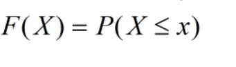
累积分布函数

对于随机变量X，当x为是实数时，F(X)叫做累积分布函数，也叫分布函数

求正态分布中随机变量小于等于3的概率：

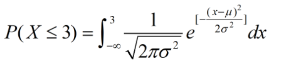
累积分布函数

stats.norm.cdf 累积分布函数。

stats.norm.cdf(loc = 4, scale = 0.8, x = 4)
#0.500

左侧概率与百分位数

数据小于等于某个值的概率就叫做左侧概率。通过累积分布函数等到。
百分位数位能得到某个概率的那个值叫做百分位数。
平均值
stats.norm.pdf正态分布概率密度函数。
stats.norm.ppf()计算百分位数
stats.norm.cdf() 累积分布函数。

stats.norm.ppf(loc = 4, scale = 0.8, q = 0.025)
#2.432

二者关系

left = stats.norm.cdf(loc = 4, scale = 0.8, x = 3)
#x=3求变量小于等于3的概率
stats.norm.ppf(loc = 4, scale = 0.8, q = left)
#3.000

stats.norm.ppf(loc = 4, scale = 0.8, q = 0.5)
#4.000

标准正态分布

均值为0，方差为1的正态分布叫做标准正态分布。

t值

统计量的计算方法:

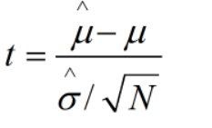
为样本均值，μ为总体均值，σ为实际样本的无偏差标准差，N为样本容量
文字描述为t值 = 样本均值-总体均值/标准误差

t值的样本分布

# 随机数种子
np.random.seed(1)
# 存放 t 值的空间
t_value_array = np.zeros(10000)
# 实例化一个正态分布
#均值为4，标准差为0.8
norm_dist = stats.norm(loc = 4, scale = 0.8)
# 开始实验
for i in range(0, 10000):
    sample = norm_dist.rvs(size = 10)
    sample_mean = sp.mean(sample)
    #求样本的标准误差
    sample_std = sp.std(sample, ddof = 1)
    sample_se = sample_std / sp.sqrt(len(sample))
    t_value_array[i] = (sample_mean - 4) / sample_se

绘制直方图

# t 值的直方图
sns.distplot(t_value_array, color = 'black')

# 标准正态分布的概率祺
x = np.arange(start = -8, stop = 8.1, step = 0.1)
plt.plot(x, stats.norm.pdf(x = x), 
         color = 'black', linestyle = 'dotted')

t分布

当总体服从正态分布时，t值得样本分布就是t分布
样本容量为N，N-1为自由度
t分布的图形与自由度有关，如果自由度为n，则t分布表示为t(n)
t分布的均差为0，t分布得均差稍大于1.
t(n)的方差=n/n-2
t分布的概率密度函数和标准正太分布的概率密度显示在同一张图上

iplt.plot(x, stats.norm.pdf(x = x), 
         color = 'black', linestyle = 'dotted')
plt.plot(x, stats.t.pdf(x = x, df = 9), 
         color = 'black')

3-2-10实现协方差矩阵

使用numpy的cov函数可以便捷地计算协方差矩阵

print(np.cov(x,y,ddof=0))
#[[ 3.2816  6.906 ]
 # [ 6.906  25.21  ]]
 #通过指定ddof=1，可以计算分母为N-1地协方差矩阵
print(np.cov(x,y,ddof=1))
# [[ 3.64622222  7.67333333]
#  [ 7.67333333 28.01111111]]

t分布的意义就是在总体方差位置时也可以研究样本均值的分布

参考资料

[日] 马场真哉 著, 吴昊天 译. 用Python动手学统计学[M]. 1. 人民邮电出版社, 2021-06-01.
菜鸟网站python3