Pytorch实现线性回归的两种方式

一、纯手写方式

既要实现线性回归，那么大致的思路是：在每一个循环的epoch里面取出真实的X和Y的值，然后使用X计算预测的Y_hat，使用平方损失函数或者其他的损失函数计算损失值，然后loss反向传播更新参数。

代码如下：

import torch
import random
# 首先导入包并定义真实的参数值
true_w = torch.tensor([2.4,3.5])
true_b = 1
# 定义合成数据的方法，需要注意的是为了更逼真一点，我们在y值后面添加了一个噪声
def synthetic_data(w,b):
    X = torch.normal(0,1,(1000,len(w)))
    y = torch.matmul(X,w) + b
    y += torch.normal(0,0.01,y.shape)
    return X,y.reshape((-1,1))
features,labels = synthetic_data(true_w,true_b)

# 定义完真实数据之后需要实现一个取数据的迭代器
def data_iter(batch_size,features,labels):
    num_examples = len(features)
    indices = list(range(num_examples))
    random.shuffle(indices)
    for i in range(0,num_examples,batch_size):
        batch_indices = torch.tensor(indices[i:min(i+batch_size,num_examples)])
    yield features[batch_indices],labels[batch_indices]

batch_size = 10

# 定义线性模型
def linreg(X,w,b):
    return torch.matmul(X,w) + b
# 定义误差计算公式
def square_loss(y_hat,y):
    return (y_hat-y.reshape(y_hat.shape))**2
# 定义更新的方式，使用SGD
def sgd(params,lr,batch_size):
    with torch.no_grad():
        for param in params:
            param -= lr*param.grad / batch_size
            param.grad.zero_()
# 开始训练，随机设置w和b
w = torch.normal(0,0.01,size=(2,1),requires_grad=True)
b = torch.zeros(1,requires_grad=True)
# 设置训练的轮数以及学习率
epochs = 5
batch_size = 10
lr = 0.1
for epoch in range(epochs):
    for X,y in data_iter(batch_size,features,labels):
        y_hat = linreg(X,w,b)
        loss = square_loss(y_hat,y)
        loss.sum().backward()
        sgd([w,b],lr,batch_size)
    with torch.no_grad():
        train_l = square_loss(linreg(features,w,b),labels)
        print(f"epoch {epoch+1},loss {float(train_l.mean())}")

最终运行结果：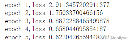
如果想进一步减小误差可以增加训练的次数也可以适当的增加学习率。

二、简洁写法
所谓的优雅一点的写法就是使用torch封装好的库，直接调用相关的库就行了
代码如下

# 导入库
import numpy as np
import torch
from torch.utils import data
# 真实参数的值
w_true = torch.tensor([2,-3.4])
b_true = 4
# 合成数据
def synthetic_data(w,b,num_examples):
    X = torch.normal(0,1,(num_examples,len(w)))
    y = torch.matmul(X,w) + b
    y += torch.normal(0,0.001,y.shape)
    return X,y.reshape(-1,1)
features,labels = synthetic_data(w_true,b_true,1000)
# 使用data生成数据迭代器
def load_array(data_arrays,batch_size,is_train=True):
    dataset = data.TensorDataset(*data_arrays)
    return data.DataLoader(dataset,batch_size,shuffle=is_train)

batch_size = 10
data_iter = load_array((features,labels),batch_size)

next(iter(data_iter))

# 网络模型，使用Sequential将模型放在容器里面
from torch import nn
net = nn.Sequential(nn.Linear(2,1))

# 容器里面的第一个就是线性模型层
# 初始化网络参数
net[0].weight.data.normal_(0,0.01)
net[0].bias.data.fill_(0)

# 使用均方误差
loss = nn.MSELoss()

# SGD优化方法
trainer = torch.optim.SGD(net.parameters(),lr = 0.03)

num_epochs = 3
for epoch in range(num_epochs):
    for X,y in data_iter:
        l = loss(net(X),y)
        trainer.zero_grad()
        l.backward()
        trainer.step()
    
    l = loss(net(features),labels)
    print(f"epoch{epoch+1},loss{l:f}")

总结：计算误差， 将优化器梯度置为0（因为pytorch梯度是默认累加的，因此每次需要将他手动置为0），误差反向传播，优化器更新参数