


目录
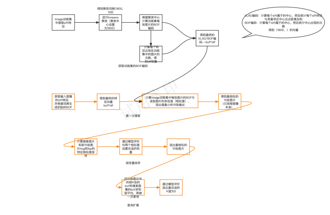
算法流程图
原项目代码+报告
ps:存储的结果的路径为作者电脑的绝对路径,所以还是要自己运行一遍
数据集:训练集在image下,测试集在test下
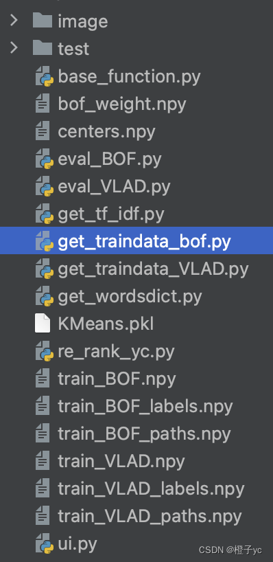
运行顺序get_wordsdict.py、get_traindata_bof.py、get_tf_idf.py
评价的文件——re_rank_yc.py
系统UI运行的文件——ui.py
代码链接
实现
方便复现——目录结构
1、获取词典
算法:提取训练集所有图片的sift特征(每张图片的sift特征128维,但个数不同),用kmeans聚类(聚类中心设置为1800)获得特征中心(即词典)保存在’centers.npy’文件中(血泪教训:不要保存为.plk格式,换个环境就会有读取问题)
ps:sift函数需要将python版本降到3.7
#获取图片的局部特征--sift特征
def get_feature(img):
    # sift = cv2.SIFT_create()
    sift = cv2.xfeatures2d.SIFT_create()
    gray = cv2.cvtColor(img, cv2.COLOR_BGR2GRAY)
    kp = sift.detect(gray, None)
    sift_val_back = sift.compute(gray, kp)[1]
    [r,c]=sift_val_back.shape
    combine = sift_val_back

#获取词典--kmeans聚类--1800
def get_wordsdict(img,SeedNum):
    Combine = []
    for i in img:
        combine= get_feature(i)
        # print(combine.shape)
        Combine.append(combine)
    Combine = np.vstack(Combine)#请节约内存!! 不要在循环里 Combine = np.vstack(Combine,combine)
    print(Combine.shape)
    # kmeans 聚类, bow[i] 为每个特征属于哪个组的, cord[i] 为各个中心组分别是第几号的
    #  distance[i] 为各个特征与所属的中心点的距离差
    model = KMeans(n_clusters=SeedNum, random_state=9)
    model.fit_transform(Combine)
    #保存码本
    #joblib.dump(model, 'KMeans.pkl')
    centers = model.cluster_centers_
    np.save('centers.npy',centers)
    print(centers.shape)#(1800, 128)

traindata, labels, paths = get_data('./image')#获取训练集‘image’下的所有文件
get_wordsdict(traindata,1800)#使用kmeans进行聚类--聚类中心个数设置为1800--结果保存到centers.npy文件中(存放聚类的中心点)
2、获取图像的BOF或VLAD特征
理论上VLAD特征准确的应该高于BOF,在车牌数据集中,感觉还是BOF表现比较好,放两个代码
#返回的为BOF向量--未做tf-idf处理
#L为1维的list--len(L)=1800
def BOF(img):
    features = get_feature(img) #输入一张图像 返回sift特征  features.shape = (X, 128)  不同图片生成的特征个数(X)不同
    centers = np.load('./centers.npy')  # 聚类的中心点  centers.shape = (1800, 128)
    wordCnt = 1800  #聚类中心个数  码本大小
    L = [0 for j in range(1800)]  #initial BOF向量 --1800长度的list
    #统计图片的features中  聚类中心出现的次数
    for i in range(0, features.shape[0]):
        #第i张图片的特征点
        fi = features[i]
        diffMat = np.tile(fi, (wordCnt, 1)) - centers
        #axis=1按行求和,即求特征到每个中心点的距离
        sqSum = (diffMat**2).sum(axis=1)
        dist = sqSum**0.5
        #升序排序
        sortedIndices = dist.argsort()
        #取出最小的距离,即找到最近的中心点
        idx = sortedIndices[0]
        #该中心点对应+1
        L[idx] += 1
    # print("get_single_bof")
    return L
def VLAD(img):
    combine = get_feature(img)
    centers = np.load('./centers.npy')#聚类的中心点
    L = [0 for j in range(1800)]

    for i in range(0, combine.shape[0]):
        #第i张图片的特征点
        fi = combine[i]
        diffMat = np.tile(fi, (1800, 1)) - centers
        #axis=1按行求和,即求特征到每个中心点的距离
        sqSum = (diffMat**2).sum(axis=1)
        dist = sqSum**0.5
        #升序排序
        sortedIndices = dist.argsort()
        #取出最小的距离,即找到最近的中心点
        idx = sortedIndices[0]
        #该中心点对应+1
        L[idx] += dist[idx]
    # print("=======get_sigle_feature_finish======")
    return l2_normalize(L)
    # return L
保存训练集的BOF特征向量
#获取data数据
def get_data(path):
    cate = []
    for i in os.listdir(os.path.abspath(path)):
        if (i[0] != '.'):
            cate.append(i)
    data = []
    labels = []
    paths = []
    for i in cate:
        for j in os.listdir(os.path.join(os.path.abspath(path), i)):
            if (j.split('.')[1] == 'jpg'):
                labels = np.append(labels, j.split('_')[0])  # 种类
                im = cv2.imread(os.path.join(os.path.abspath(path), i, j),cv2.IMREAD_COLOR)  # 读取图片
                data.append(im)
                paths = np.append(paths, os.path.join(os.path.join(os.path.abspath(path), i), j))

    return data,labels,paths


# 完成获取码本、训练集BOF特征
traindata, labels, paths = get_data('./image')
print("=============get_image_finish=============")
    # 获取训练集的BOF特征
train_BOf_vector = []
for i in traindata:
    train_BOf_vector.append(BOF(i))
print("==========finish=========")


 np.save("./train_BOF.npy",train_BOf_vector)
 np.save("./train_BOF_labels.npy",labels)
 np.save("./train_BOF_paths",paths)
3、ti-idf优化
算法思想:统计每个特征(对应词典–也就是聚类的1800个特征中心)在训练集中出现的次数(比如一个特征在15张图片中存在,则该特征对应的值为15),得到一个1800长度的一维向量。并保存为"bof_weight.npy"
import numpy as np
import math
#计算公式  hj = log(n/fj)
# ---n为训练集所有图片数量
# ---fj为第j个聚类特征在训练集中出现的图片数量
# ---hj为j向量的权重
def get_tf_idf():
    train_bof = np.load('./train_BOF.npy')
    # print(train_bof.shape)  #(946, 1800)
    N = train_bof.shape[0]#训练集中的图片总数
    f = [0 for j in range(1800)]  #生成码本的 权重向量
    #计算每个特征出现的图片次数
    for i in range(train_bof.shape[0]):
        for j in range(train_bof.shape[1]):
            if(train_bof[i][j]!=0):
                f[j]+=1;
    # print(len(f)) #1800
    for i in range(len(f)):
        f[i]=math.log(N/f[i])
    # print(f)
    np.save("bof_weight.npy",f)
4、得到初步的结果
函数说明:输入搜索图片的路径,返回最相似的15张图片(由于作者采用的训练集包括了测试集图片,所以查询16张,将查询到的最相似的一张图片(其本身)排除)
算法:提取搜索图片的sift特征,结合之前获取到的词典得到BOF特征向量,计算训练集中每张图片的BOF向量和该特征向量的余弦相似度(越相似,值越小),得到最终的排序结果。
def get_ans(path):
    # #----------------使用VLAD--------------
    # im = cv2.imread(path)
    # im_vlad = VLAD(im)
    # train_VLAD = np.load('./train_VLAD.npy')
    # train_labels = np.load('./train_VLAD_labels.npy')
    # train_path = np.load('./train_VLAD_paths.npy')
    # idf = np.load('./bof_weight.npy')  #tf-idf 的bof权重
    # tf= train_VLAD
    # train_VLAD = tf*idf
    # im_vlad = im_vlad*idf
    #
    # zj = []
    # k=16
    # for i in train_VLAD:
    #     zj.append(np.dot(i, im_vlad) / (np.linalg.norm(i) * np.linalg.norm(im_vlad)))
    # index = np.argsort(zj)[::-1][0:k]#倒序--对应Coslength函数
    # return train_path[index][1:-1]

    #----------------使用BOF------------
    im = cv2.imread(path)
    im_Bof = BOF(im)
    train_BOF = np.load('./train_BOF.npy')
    train_labels = np.load('./train_BOF_labels.npy')
    train_path = np.load('./train_BOF_paths.npy')
    idf = np.load('./bof_weight.npy')  #tf-idf 的bof权重
    train_bof_final = train_BOF*idf
    im_Bof = (im_Bof)*idf

    # print(train_bof_final.shape) #(946, 1800)
    zj = []
    k=16
    for i in train_bof_final:
        # zj.append(calEuclidean(i, im_Bof))  # 欧式距离--越小越相似
        zj.append(np.dot(i, im_Bof) / (np.linalg.norm(i) * np.linalg.norm(im_Bof)))
    index = np.argsort(zj)[::-1][0:k]#倒序--对应Coslength函数
    # index = np.argsort(zj)[0:k]
    #去除其本身
    return train_path[index][1:-1]
5、re-rank重排序优化
函数:输入查询图片的路径path1,和初始查询得到的15张图片的地址path
算法思想:选择线性重排序实现,选取了边缘特征和纹理特征(hog和lbp),分别计算15张图片和搜索图片的hog、lbp的余弦相似度向量,将两个向量赋予权重,得到最终结果。
ps:比较手笨,手动根据评价选择了最优的权重为0.5和0.6
结果展示:
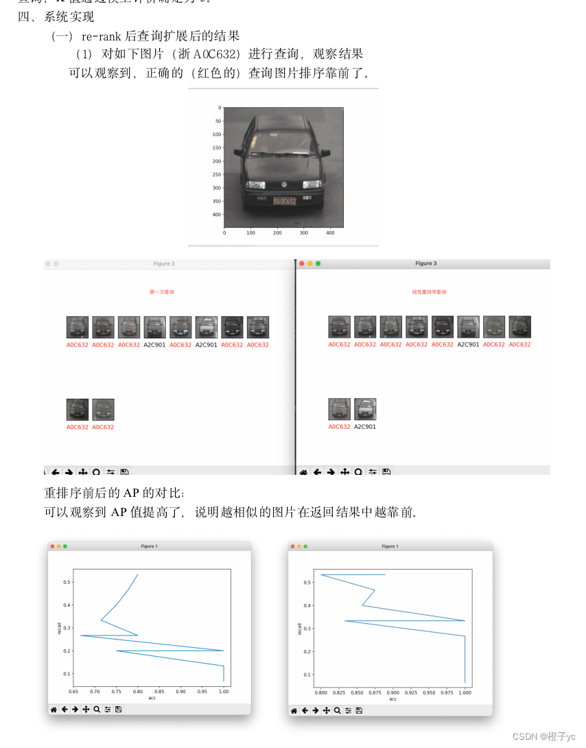
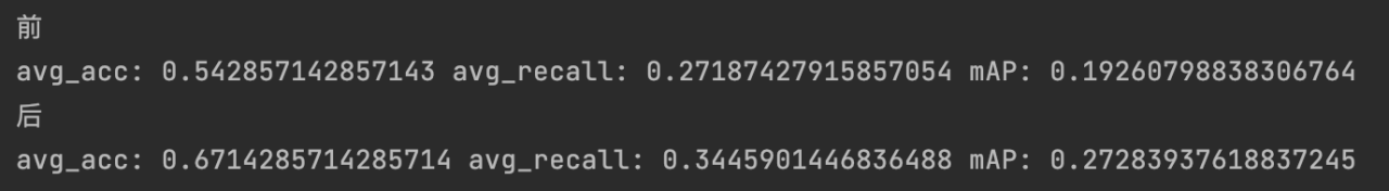
(2)总体的acc、recall和mAP 相较于未重排序的查询有所提高:
def get_hog(path):

    # 打印特征向量的长度
    # print(feat.shape)
    img = cv2.imread(path)
    # img1 = cv2.resize(img, (300, 300))
    image2 = cv2.cvtColor(img, cv2.COLOR_BGR2GRAY)
    ft = hog(image2, orientations=9,  # 将180°划分为9个bin,20°一个
                       pixels_per_cell=(8, 8),  # 每个cell有8*8=64个像素点
                       cells_per_block=(8, 8),  # 每个block中有8*8=64个cell
                       block_norm='L2-Hys',  # 块向量归一化 str {‘L1’, ‘L1-sqrt’, ‘L2’, ‘L2-Hys’}
                       transform_sqrt=True,  # gamma归一化
                       feature_vector=True  # 转化为一维向量输出
                        )  # 输出HOG图像
    return ft
#path为初始查询返回的结果的图像的路径(get_ans)


def get_lbp(path):
    image = cv2.imread(path)
    image1 = cv2.cvtColor(image, cv2.COLOR_BGR2GRAY)
    radius = 3  # LBP算法中范围半径的取值
    n_points = 8 * radius  # 领域像素点数
    lbp = local_binary_pattern(image1, n_points, radius)

    arr = lbp.flatten()  # 二维数组序列化成一维数组
    return arr
def get_lbp_simi(path,path1):
    zj = []
    test = get_lbp(path1)
    train = []
    for i in path:
        train.append(get_lbp(i))
    for i in train:
        zj.append(np.dot(i, test) / (np.linalg.norm(i) * np.linalg.norm(test)))
    return zj  #返回相似度  越小越相似
def get_hog_simi(path,path1):
    zj = []
    test = get_hog(path1)
    train = []
    for i in path:
        train.append(get_hog(i))
    for i in train:
        zj.append(np.dot(i, test) / (np.linalg.norm(i) * np.linalg.norm(test)))
    return zj  #返回相似度  越小越相似
def re_rank(path1,path,k):
    # path1 = './test/A0C573/A0C573_20151103073308_3029240562.jpg'
    #re-rank重排序
    simi1 = get_hog_simi(path, path1)
    simi2 = get_lbp_simi(path, path1)
    # simi1,simi2 = get_simi(path,path1)
    simi1=np.array(simi1)
    simi2=np.array(simi2)
    simi = simi1*0.5+simi2*0.6
    index = np.argsort(simi)[::-1][0:k]  # 倒序--对应Coslength函数
    ans = path[index]
    return ans#返回路径
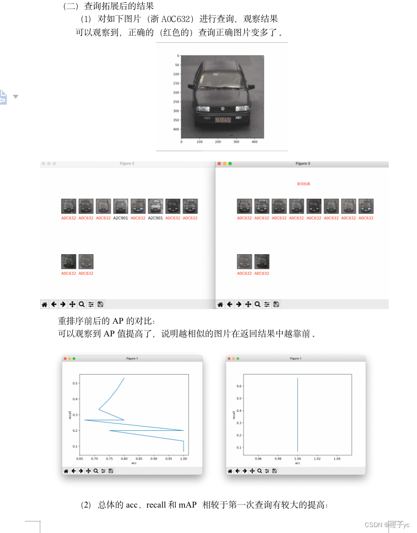
6、查询拓展
思想:选取re-rank后的前K张图片的bof特征和查询图片的bof特征求平均值,再做一次初始查询。
实验结果:K选取5最优
结果展示:
def requery(path1,path,k,k1):
    idf = np.load('./bof_weight.npy')  # tf-idf 的bof权重
    im = cv2.imread(path1)
    im_Bof = BOF(im)
    bof_test = (im_Bof) * idf
    #对查询结果path+图像本身path1的特征求和取平均,再做一次查询
    count = 0
    for i in path:
        if(count==k):#表中top@K表示取前K个样本求和取平均。
            break
        count=count+1
        im = cv2.imread(i)
        im_Bof = BOF(im)
        im_Bof = (im_Bof) * idf
        for j in range(len(bof_test)):
            bof_test[j]=bof_test[j]+im_Bof[j]
    for i in range(len(bof_test)):
        bof_test[i]=bof_test[i]/(len(path)+1)

    #重新查询
    train_BOF = np.load('./train_BOF.npy')
    train_path = np.load('./train_BOF_paths.npy')
    idf = np.load('./bof_weight.npy')  #tf-idf 的bof权重
    train_bof_final = train_BOF*idf

    zj = []
    for i in train_bof_final:
        zj.append(np.dot(i, bof_test) / (np.linalg.norm(i) * np.linalg.norm(bof_test)))
    index = np.argsort(zj)[::-1][0:k1]  # 倒序--对应Coslength函数
    ans = train_path[index]
    # show_ans(path[0:10])
    # show_ans(ans)
    # plt.show()
    return ans #返回结果图片存放地址
7、最终结果
函数:输入查询图片的路径path1,初始查询结果数量设置为k1=15,重排序选取查询结果数量设置为k=10
def get_final_ans(path1,k1,k):#首次查询查k1张图片;重排序查询k张;返回查询k1张图像的结果
    path = get_ans(path1)#选15张初始查询图片
    ans1 = re_rank(path1,path,10)#对15张重排序 选出10张作为输出结果
    ans = requery(path1,ans1,k,k1) #对重排序结果 提取前k张结果对特征求平均 用新特征 重新查询k1张图像
    return ans
8、评价
比较初始查询结果和re-rank、查询拓展之后结果的avg_acc、avg_recall、mAP对比
单张图片评价
def ceshi_single(path1,Np):
    path = get_ans(path1)#初始查询15张
    print(path1)
    #评价
    # 前
    acc = compu_acc(path[0:10], path1, 10)#选择15张中的前10张
    recall = compu_recall(acc*10,Np)
    AP = show_ROC(path[0:10], path1, Np)
    print('acc:', acc, 'recall:', recall, 'AP', AP)

    # re-rank+拓展查询后
    ans = get_final_ans(path1,10, 5)#首次查询15张 重排序选出15张 拓展查询 选出前5张取特征平均 重新查询15张结果
    acc1 = compu_acc(ans, path1, 10)
    recall1 = compu_recall(acc1*10,Np)
    AP1 = show_ROC(ans,  path1, Np)


    print('acc:', acc1, 'recall:', recall1, 'AP', AP1)
    return acc,recall,AP,acc1,recall1,AP1,path,ans

#单张图片查询测试
path1 = './test/A0C632/A0C632_20151103114000_6597334762.jpg'
Np = 0
train_labels = np.load('./train_BOF_labels.npy')
for i in train_labels:
   if (path1.split('/')[-2] == i):
       Np += 1
print(Np)
acc,recall,mAP,acc1,recall1,mAP1,path,ans = ceshi_single(path1,Np)
plt.imshow(cv2.imread(path1))
show_ans(path[0:10],path1)
show_ans(ans,path1)
plt.show()
测试集的评价
def cheshi():
#计算整个数据集的acc
testdata, test_labels, test_path = get_data('./test')
avg_acc1=0
avg_acc2=0
avg_recall1=0
avg_recall2=0
avg_mAP1 = 0
avg_mAP2 =0
for path1 in test_path:
# 计算召回率
Np = 0;
train_labels = np.load('./train_BOF_labels.npy')
for i in train_labels:
if (path1.split('/')[-2] == i):
Np += 1
acc, recall, mAP, acc1, recall1, mAP1,c,a = ceshi_single(path1,Np)
avg_acc1 = avg_acc1 + acc
avg_recall1 = avg_recall1 + recall
avg_mAP1 = avg_mAP1 + mAP
avg_acc2 = avg_acc2 + acc1
avg_recall2 = avg_recall2 + recall1
avg_mAP2 = avg_mAP2 + mAP1
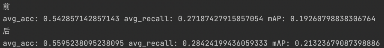
print('前')
print('avg_acc:',avg_acc1/len(test_path),'avg_recall:',avg_recall1/len(test_path),'mAP:',avg_mAP1/len(test_path))
print('后')
print('avg_acc:',avg_acc2/len(test_path),'avg_recall:',avg_recall2/len(test_path),'mAP:',avg_mAP2/len(test_path))
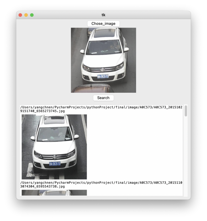
9、系统
ui系统界面展示
from pathlib import Path
from PIL import Image, ImageTk
import tkinter as tk
from tkinter.constants import *
from tkinter.scrolledtext import ScrolledText
import tkinter.filedialog
import cv2
from get_traindata_VLAD import VLAD
from get_traindata_bof import BOF
from base_function import calEuclidean,Coslength
import numpy as np
from sklearn.cluster import KMeans
import cv2
import numpy as np
import matplotlib.pyplot as plt
import math
from skimage.feature import local_binary_pattern
from base_function import get_data,calEuclidean
from get_traindata_bof import BOF
from sklearn.cluster import KMeans
from skimage.feature import hog


#采用线性组合算法 对初始排序结果的图像提取hog和lbp特征直方图 适用余弦相似度计算图像特征值的相似值,采用0.5 0.5的权重重排序
#从初始15张排序结果 选出10张重排序结果输出
#实验结果表明,有些图像的acc和recall值会增大或减小,但mAP大多数是增大的


def get_hog(path):

    # 打印特征向量的长度
    # print(feat.shape)
    img = cv2.imread(path)
    # img1 = cv2.resize(img, (300, 300))
    image2 = cv2.cvtColor(img, cv2.COLOR_BGR2GRAY)
    ft = hog(image2, orientations=9,  # 将180°划分为9个bin,20°一个
                       pixels_per_cell=(8, 8),  # 每个cell有8*8=64个像素点
                       cells_per_block=(8, 8),  # 每个block中有8*8=64个cell
                       block_norm='L2-Hys',  # 块向量归一化 str {‘L1’, ‘L1-sqrt’, ‘L2’, ‘L2-Hys’}
                       transform_sqrt=True,  # gamma归一化
                       feature_vector=True  # 转化为一维向量输出
                        )  # 输出HOG图像
    return ft
#path为初始查询返回的结果的图像的路径(get_ans)


def get_lbp(path):
    image = cv2.imread(path)
    image1 = cv2.cvtColor(image, cv2.COLOR_BGR2GRAY)
    radius = 3  # LBP算法中范围半径的取值
    n_points = 8 * radius  # 领域像素点数
    lbp = local_binary_pattern(image1, n_points, radius)

    arr = lbp.flatten()  # 二维数组序列化成一维数组
    return arr
def get_lbp_simi(path,path1):
    zj = []
    test = get_lbp(path1)
    train = []
    for i in path:
        train.append(get_lbp(i))
    for i in train:
        zj.append(np.dot(i, test) / (np.linalg.norm(i) * np.linalg.norm(test)))
    return zj  #返回相似度  越小越相似
def get_hog_simi(path,path1):
    zj = []
    test = get_hog(path1)
    train = []
    for i in path:
        train.append(get_hog(i))
    for i in train:
        zj.append(np.dot(i, test) / (np.linalg.norm(i) * np.linalg.norm(test)))
    return zj  #返回相似度  越小越相似

def re_rank(path1,path,k):
    # path1 = './test/A0C573/A0C573_20151103073308_3029240562.jpg'
    #re-rank重排序
    simi1 = get_hog_simi(path, path1)
    simi2 = get_lbp_simi(path, path1)
    # simi1,simi2 = get_simi(path,path1)
    simi1=np.array(simi1)
    simi2=np.array(simi2)
    simi = simi1*0.5+simi2*0.6
    index = np.argsort(simi)[::-1][0:k]  # 倒序--对应Coslength函数
    ans = path[index]
    return ans
def requery(path1,path,k,k1):
    idf = np.load('./bof_weight.npy')  # tf-idf 的bof权重
    im = cv2.imread(path1)
    im_Bof = BOF(im)
    bof_test = (im_Bof) * idf
    #对查询结果path+图像本身path1的特征求和取平均,再做一次查询
    count = 0
    for i in path:
        if(count==k):#表中top@K表示取前K个样本求和取平均。
            break
        count=count+1
        im = cv2.imread(i)
        im_Bof = BOF(im)
        im_Bof = (im_Bof) * idf
        for j in range(len(bof_test)):
            bof_test[j]=bof_test[j]+im_Bof[j]
    for i in range(len(bof_test)):
        bof_test[i]=bof_test[i]/(len(path)+1)

    #重新查询
    train_BOF = np.load('./train_BOF.npy')
    train_path = np.load('./train_BOF_paths.npy')
    idf = np.load('./bof_weight.npy')  #tf-idf 的bof权重
    train_bof_final = train_BOF*idf

    zj = []
    for i in train_bof_final:
        zj.append(np.dot(i, bof_test) / (np.linalg.norm(i) * np.linalg.norm(bof_test)))
    index = np.argsort(zj)[::-1][0:k1]  # 倒序--对应Coslength函数
    ans = train_path[index]
    # show_ans(path[0:10])
    # show_ans(ans)
    # plt.show()
    return ans #返回结果图片存放地址

def get_final_ans(path1,k1,k):#首次查询查k1张图片;重排序查询k张;返回查询k1张图像的结果
    path = get_ans(path1)#选15张初始查询图片
    ans1 = re_rank(path1,path,10)#对15张重排序 选出10张作为输出结果
    ans = requery(path1,ans1,k,k1) #对重排序结果 提取前k张结果对特征求平均 用新特征 重新查询k1张图像
    return ans
def get_ans_(path):
    return get_final_ans(path,10, 5)
#获取给定图片的15张最相似图片的路径
def get_ans(path):
    # #----------------使用VLAD--------------
    # im = cv2.imread(path)
    # im_vlad = VLAD(im)
    # train_VLAD = np.load('./train_VLAD.npy')
    # train_labels = np.load('./train_VLAD_labels.npy')
    # train_path = np.load('./train_VLAD_paths.npy')
    # idf = np.load('./bof_weight.npy')  #tf-idf 的bof权重
    # tf= train_VLAD
    # train_VLAD = tf*idf
    # im_vlad = im_vlad*idf
    #
    # zj = []
    # k=16
    # for i in train_VLAD:
    #     zj.append(np.dot(i, im_vlad) / (np.linalg.norm(i) * np.linalg.norm(im_vlad)))
    # index = np.argsort(zj)[::-1][0:k]#倒序--对应Coslength函数
    # return train_path[index][1:-1]

    #----------------使用BOF------------
    im = cv2.imread(path)
    im_Bof = BOF(im)
    train_BOF = np.load('./train_BOF.npy')
    train_labels = np.load('./train_BOF_labels.npy')
    train_path = np.load('./train_BOF_paths.npy')
    idf = np.load('./bof_weight.npy')  #tf-idf 的bof权重
    train_bof_final = train_BOF*idf
    im_Bof = (im_Bof)*idf

    # print(train_bof_final.shape) #(946, 1800)
    zj = []
    k=16
    for i in train_bof_final:
        # zj.append(calEuclidean(i, im_Bof))  # 欧式距离--越小越相似
        zj.append(np.dot(i, im_Bof) / (np.linalg.norm(i) * np.linalg.norm(im_Bof)))
    index = np.argsort(zj)[::-1][0:k]#倒序--对应Coslength函数
    # index = np.argsort(zj)[0:k]
    #去除其本身
    return train_path[index][1:-1]


class App:
    def __init__(self, image_file_extensions):
        self.root = tk.Tk()
        self.image_paths = []
        self.image_file_extensions = image_file_extensions
        self.create_widgets()
        self.root.mainloop()


    def create_widgets(self):
        self.list_btn = tk.Button(self.root, text='Chose_image', command=self.chose_image)
        self.list_btn.grid(row=0, column=0)


        self.label = tk.Label(self.root)
        self.label.grid(row=1,column=0)

        self.show_btn = tk.Button(self.root, text='Search', command=self.show_images)
        self.show_btn.grid(row=2, column=0)

        self.text = ScrolledText(self.root, wrap=WORD)
        self.text.grid(row=3, column=0, padx=10, pady=10)

        self.text.image_filenames = []
        self.text.images = []

    def chose_image(self):
        path = tk.filedialog.askopenfilename()
        img = Image.open(path)
        h = int(img.size[0]*0.5)
        w = int(img.size[1]*0.5)
        img = Image.open(path).resize((h,w))
        img = ImageTk.PhotoImage(img)
        self.label.image = img
        self.label.config(image=img)
        self.label.image = img
        self.image_paths.clear()
        # for i in get_ans_VLAD(path):
        #     self.image_paths.append(i)
        for i in get_ans_(path):
            self.image_paths.append(i)

    def list_images(self):  #结果图片的路径
        ''' Create and display a list of the images the in folder that have one
            of the specified extensions. '''
        self.text.image_filenames.clear()
        # for filepath in Path(self.image_folder_path).iterdir():
        #     if filepath.suffix in self.image_file_extensions:
        #         self.text.insert(INSERT, filepath.name+'\n')
        #         self.text.image_filenames.append(filepath)
        for i in self.image_paths:
            self.text.insert(INSERT, i + '\n')
            self.text.image_filenames.append(i)
        # for filepath in self.image_paths:
        #     self.text.insert(INSERT, filepath + '\n')
        #     self.text.image_filenames.append(filepath)

    def show_images(self):
        self.list_images()
        ''' Show the listed image names along with the images themselves. '''
        self.text.delete('1.0', END)  # Clear current contents.
        self.text.images.clear()
        # Display images in Text widget.
        for image_file_path in self.text.image_filenames:
            img = Image.open(image_file_path)
            h = int(img.size[0] * 0.5)
            w = int(img.size[1] * 0.5)
            img = Image.open(image_file_path).resize((h, w))
            img = ImageTk.PhotoImage(img)

            # self.text.insert(INSERT, image_file_path.name+'\n')
            self.text.insert(INSERT, image_file_path+'\n')
            self.text.image_create(INSERT, padx=5, pady=5, image=img)
            self.text.images.append(img)  # Keep a reference.
            self.text.insert(INSERT, '\n')

if __name__ == '__main__':
    #ui显示
    image_file_extensions = {'.jpg', '.png'}
    App(image_file_extensions)


 被折叠的 条评论
为什么被折叠?
被折叠的 条评论
为什么被折叠?
 到【灌水乐园】发言


