


吴恩达机器学习作业四:BP神经网络


1.1 Visualizing the data
这与上一个练习中使用的数据集相同。ex3data1.mat中有5000个训练示例,其中每个训练示例是数字的20像素乘20像素灰度图像。每个像素由一个浮点数表示,表示该位置的灰度强度。像素的20乘20网格被“展开”成400维向量。这些训练示例中的每一个都成为我们的数据矩阵X中的一行。这给了我们一个5000×400的矩阵X,其中每一行都是手写数字图像的训练示例。
训练集的第二部分是包含训练集标签的5000维向量y。为了使事情更兼容八进制/MATLAB索引,在没有零索引的情况下,我们将数字零映射到值10。因此,“0”数字标记为“10”,而数字“1”到“9”按其自然顺序标记为“1”到“9”。
#coding=utf-8
import numpy as np
import pandas as pd
from scipy.io import loadmat
import scipy.optimize as opt
from matplotlib import pyplot as plt
from sklearn.metrics import classification_report  # 这个包是评价报告

def load_data(path):
    data = loadmat(path)
    x = data['X']
    y = data['y']
    return x,y

path_data = 'D:\编程\ex3data1.mat'

x1,y1= load_data(path_data)
print(x1.shape,y1.shape)


# 随机画100个数字
def plot_images(x):
    pick_index = np.random.choice(x.shape[0],100)
    pick_images = x[pick_index,:]  #(100,400)
    fig, ax = plt.subplots(nrows=10, ncols=10, sharey=True, sharex=True, figsize=(8, 8))
    for i in range(10):
        for j in range(10):
            # fig, ax = plt.subplots()等价于:
            # fig = plt.figure()
            # ax = fig.add_subplot(1, 1, 1)
            ax[i,j].matshow(pick_images[10*i+j,:].reshape(20,20))
            plt.xticks([])
            plt.yticks([])
    plt.show()


print(plot_images(x1))

1.2 Model representation 模型表示
我们的网络有三层,输入层,隐藏层,输出层。我们的输入是数字图像的像素值,因为每个数字的图像大小为20*20,所以我们输入层有400个单元(这里不包括总是输出要加一个偏置单元)。

1.2.1 获取输入变量
# 获取输入变量x
x1 = np.insert(x1,0,values=1,axis=1)
print(x1.shape)
首先我们要将标签值(1,2,3,4,…,10)转化成非线性相关的向量,向量对应位置(y[i-1])上的值等于1,例如y[0]=6转化为y[0]=[0,0,0,0,0,1,0,0,0,0]。
# 获取输入变量y
y1_new = []
for i in y1:
    y_array = np.zeros(10)
    y_array[i-1] = 1
    y1_new.append(y_array)
y1_new = np.array(y1_new)
print(y1_new.shape)
# (500,10)
方法二,也可对y标签进行one hot编码,如下。
from sklearn.preprocessing import OneHotEncoder
encoder  = OneHotEncoder(sparse=False)
y1_new = encoder.fit_transform(y1)
print(y1_new.shape)
1.2.2 获取权重参数
我们已经向您提供了一组网络参数θ1和θ2,这些参数已经过我们的培训。它们存储在ex4weights.mat将由ex4.m加载到θ1和θ2。这些参数的维数是为第二层有25个单元和10个输出单元(对应于10位类)的神经网络确定的。
# 获取权重
path_theta = 'D:\编程\ex3weights.mat'
theta = loadmat(path_theta)
theta1 = theta['Theta1']  # (25, 401)
theta2 = theta['Theta2']  # (10, 26)
print(theta1.shape)
print(theta2.shape)
当我们使用高级优化方法来优化神经网络时,我们需要将多个参数矩阵展开,才能传入优化函数,然后再恢复形状。
# 序列化权重参数:将θ1和θ2合并转化为一维数组
def serialize(a,b):
    return np.append(a.flatten(),b.flatten())
theta_serialize = serialize(theta1,theta2)
print(theta_serialize.size)

# 解序列化权重参数
def deserialize(a,b):
    theta1 = serialize(a,b)[:25*401].reshape(25,401)
    theta2 = deserialize(a,b)[25*401:].reshape(10,26)
    return theta1,theta2
1.3 Feedforward and cost function
1.3.1 Feedforward
确保每层的单元数,注意输出时加一个偏置单元,s(1)=400+1,s(2)=25+1,s(3)=10。

# 前向传播
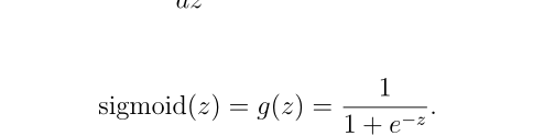
def sigmoid(z):
return 1/(1+np.exp(-z))
def feedforword(x,theta):
t1,t2 = deserialize(theta)
# 前面已经插入过偏执单元,这里就不用插入了
a1 = x
z2 = a1 @ t1.T
a2 = np.insert(sigmoid(z2),0,values=1,axis = 1)
z3 = a2 @ t2.T
a3 = sigmoid(z3)
return a1,z2,a2,z3,a3
a1,z2,a2,z3,h = feedforword(x1_new,theta_serialize)
print(a1,z2,a2,z3,h)
1.3.2 Cost function

# 无正则化代价函数
def costfunction( theta,x,y):
    a1, z2, a2, z3, h = feedforword( theta,x)
    J = - np.sum(y * np.log(h) + (1-y) * np.log(1-h))/len(x)
    return J
print(costfunction(theta_serialize,x1_new,y1_new))
# 0.2876291651613189
1.4 Regularized cost function

注意不要将每层的偏置项正则化。

# 有正则化代价函数
def regular_costf(theta,x,y,lam):
    t1,t2 = deserialize(theta)
    # 注意这里是从 1 开始
    part1 = np.sum(np.power(t1[:,1:],2))
    part2 = np.sum(np.power(t2[:,1:],2))
    reg = lam * (part1+part2) / (2*len(x))
    return costfunction(theta,x,y) + reg

print(regular_costf(theta_serialize,x1_new,y1_new,1))
# 0.38376985909092365
2 Backpropagation 反向传播
在这部分练习中,您将实现反向传播算法来计算神经网络代价函数的梯度。您需要完成nnCostFunction.m,以便它为grad返回适当的值。一旦你计算了梯度,你就可以通过使用诸如fmincg之类的高级优化器最小化代价函数J(Θ)来训练神经网络。您将首先实现反向传播算法来计算(未规范化)神经网络参数的梯度。
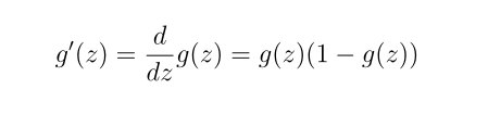
2.1 Sigmoid gradient
# sigmoid gradient  对z求偏导
def sigmoid_gradient(z):
    return sigmoid(z) * (1-sigmoid(z))
2.2 Random initialization
当我们训练神经网络时,随机初始化参数是很重要的,可以打破数据的对称性。一个有效的策略是在均匀分布(−e,e)中随机选择值,我们可以选择 e = 0.12 这个范围的值来确保参数足够小,使得训练更有效率。
# 随机初始化
def random_init(size):
    # 服从均匀分布的范围中随机返回size大小的值
    return np.random.uniform(-0.12,0.12,size)
2.3 Backpropagation


目标:获取整个网络代价函数的梯度。以便在优化算法中求解。
这里面一定要理解正向传播和反向传播的过程,才能弄清楚各种参数在网络中的维度,切记。比如手写出每次传播的式子。
# 检查一下各参数的维度

print('a1', a1.shape,'t1', t1.shape)
print('z2', z2.shape)
print('a2', a2.shape, 't2', t2.shape)
print('z3', z3.shape)
print('a3', h.shape)


# 反向传播梯度下降
def gradient(theta,x,y):
    t1,t2 = deserialize(theta)
    a1, z2, a2, z3, h = feedforword(theta, x)
    d3 = h - y #(5000,10)
    d2 = d3 @ t2[:,1:] * sigmoid_gradient(z2) #(5000,25)
    D2 = d3.T @ a2  # (10,26)
    D1 = d2.T @ a1 # (25,401)
    D = (1 / len(x)) * serialize(D1,D2)  # (1025,)
    return D
2.4 Gradient checking 梯度检测
在你的神经网络,你是最小化代价函数J(Θ)。执行梯度检查你的参数,你可以想象展开参数Θ(1)Θ(2)成一个长向量θ。通过这样做,你能使用以下梯度检查过程。


# 梯度检测
def gradient_cheecking(theta,x,y,e):
    def a_numeric_grad(plus,minus):
        # 对每个参数theta计算数值梯度,即理论梯度
        return (costfunction(plus,x,y) - costfunction(minus,x,y)) / (e * 2)
    numeric_grad = []
    for i in range(len(theta)):
        plus = theta.copy()
        minus = theta.copy()
        plus[i] = plus[i] + e
        minus[i] = minus[i] - e
        grad_i = a_numeric_grad(plus,minus)
        numeric_grad.append(grad_i)
    numeric_grad = np.array(numeric_grad)
    analytic_grad = regularized_gradient(theta,x,y)

    diff = np.linalg.norm(numeric_grad - analytic_grad) / np.linalg.norm(numeric_grad + analytic_grad)
    print(
        'If your backpropagation implementation is correct,\nthe relative difference will be smaller than 10e-9 (assume epsilon=0.0001).\nRelative Difference: {}\n'.format(
            diff))
gradient_checking(theta, X, y, epsilon= 0.0001)#这个运行很慢,谨慎运行
2.5 Regularized Neural Networks
成功实现反向传播算法后,将向梯度添加正则化。为了说明正则化,可以在使用反向传播计算梯度之后将其作为附加项添加。
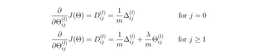
注意,你不应该正则化用来表示偏差项。此外,在参数中,i 从1开始索引,j 从0开始索引。

# 有正则化的梯度下降
def regularized_gradient(theta,x,y,lam):
    # 不惩罚偏执单元的参数
    D1,D2 = deserialize(gradient(theta,x,y))

    t1[:,0] = 0
    t2[:,0] = 0
    reg_D1 = D1 + (lam / len(x)) * t1
    reg_D2 = D2 + (lam / len(x)) * t2
    return serialize(reg_D1,reg_D2)
2.6 Learning parameters using fmincg
# 最优化函数
def nn_training(x,y):
    init_theta = random_init(10285) # 25*401+10*26
    result = opt.minimize(fun=regular_costf,x0 = init_theta,args=(x,y,1),method='TNC',jac = regularized_gradient,options={'maxiter':400})
    # 可选项:最大迭代次数,选择为300次
    return result
result = nn_training(x1_new,y1_new)
print(result)

# 计算精度
_, _, _, _, h = feedforword(result.x, x1_new)
y_pred = np.argmax(h, axis=1) + 1
print(classification_report(y1,y_pred))

# 方法二:计算精度
correct = [1 if a==b else 0 for (a,b) in zip(y1,y_pred)]
accuracy = sum(map(float,correct)) / float(len(correct))
print('accuracy = {}%'.format(accuracy * 100))

3 Visualizing the hidden layer

# 可视化隐藏层
def plot_hidden(theta):
    t1, _ = deserialize(theta)
    t1 = t1[:, 1:]  # (25,400)
    fig,ax_array = plt.subplots(5, 5, sharex=True, sharey=True, figsize=(6,6))
    for row in range(5):
        for column in range(5):
            ax_array[row, column].matshow(t1[row * 5 + column].reshape(20, 20), cmap='gray_r')
            plt.xticks([])
            plt.yticks([])
    plt.show()

plot_hidden(result.x)

以下为完整代码:
#coding=utf-8
import numpy as np
import pandas as pd
from scipy.io import loadmat
import scipy.optimize as opt
from matplotlib import pyplot as plt
from sklearn.metrics import classification_report  # 这个包是评价报告

def load_data(path):
    data = loadmat(path)
    x = data['X']
    y = data['y']
    return x,y

path_data = 'D:\编程\ex3data1.mat'

x1,y1= load_data(path_data)
print(x1.shape,y1.shape)
print(y1)


# # 随机画100个数字
# def plot_images(x):
#     pick_index = np.random.choice(x.shape[0],100)
#     pick_images = x[pick_index,:]  #(100,400)
#     fig, ax = plt.subplots(nrows=10, ncols=10, sharey=True, sharex=True, figsize=(8, 8))
#     for i in range(10):
#         for j in range(10):
#             # fig, ax = plt.subplots()等价于:
#             # fig = plt.figure()
#             # ax = fig.add_subplot(1, 1, 1)
#             ax[i,j].matshow(pick_images[10*i+j,:].reshape(20,20))
#             plt.xticks([])
#             plt.yticks([])
#     plt.show()
# print(plot_images(x1))


# 获取输入变量x
x1_new = np.insert(x1,0,values=1,axis=1)
print(x1_new.shape)


# 获取输入变量y
y1_new = []
for i in y1:
    y_array = np.zeros(10)
    y_array[i-1] = 1
    y1_new.append(y_array)
y1_new = np.array(y1_new)
print(y1_new.shape)

# 方法二:one hot 编码
from sklearn.preprocessing import OneHotEncoder
encoder  = OneHotEncoder(sparse=False)
y1_new = encoder.fit_transform(y1)
print(y1_new.shape)

# 获取权重
path_theta = 'D:\编程\ex3weights.mat'
theta = loadmat(path_theta)
theta1 = theta['Theta1']  # (25, 401)
theta2 = theta['Theta2']  # (10, 26)
print(theta1.shape)
print(theta2.shape)

# 序列化权重参数:将θ1和θ2合并转化为一维数组
def serialize(a,b):
    return np.append(a.flatten(),b.flatten())
theta_serialize = serialize(theta1,theta2)
print(theta_serialize.size)

# 解序列化权重参数
def deserialize(theta_serialize):
    theta1 = theta_serialize[:25*401].reshape(25,401)
    theta2 = theta_serialize[25*401:].reshape(10,26)
    return theta1,theta2

# 前向传播
def sigmoid(z):
    return 1/(1+np.exp(-z))

def feedforword(theta,x):
    t1,t2 = deserialize(theta)
    # 前面已经插入过偏执单元,这里就不用插入了
    a1 = x
    z2 = a1 @ t1.T
    a2 = np.insert(sigmoid(z2),0,values=1,axis = 1)
    z3 = a2 @ t2.T
    a3 = sigmoid(z3)
    return a1,z2,a2,z3,a3

a1,z2,a2,z3,h = feedforword(theta_serialize,x1_new,)
print(a1,z2,a2,z3,h)


# 无正则化代价函数
def costfunction( theta,x,y):
    a1, z2, a2, z3, h = feedforword( theta,x)
    J = - np.sum(y * np.log(h) + (1-y) * np.log(1-h))/len(x)
    return J
print(costfunction(theta_serialize,x1_new,y1_new))


# 有正则化代价函数
def regular_costf(theta,x,y,lam):
    t1,t2 = deserialize(theta)
    # 注意这里是从1 开始
    part1 = np.sum(np.power(t1[:,1:],2))
    part2 = np.sum(np.power(t2[:,1:],2))
    reg = lam * (part1+part2) / (2*len(x))
    return costfunction(theta,x,y) + reg
print(regular_costf(theta_serialize,x1_new,y1_new,1))

# 反向传播
# sigmoid gradient  对z求偏导
def sigmoid_gradient(z):
    return sigmoid(z) * (1-sigmoid(z))

# 随机初始化
def random_init(size):
    # 服从均匀分布的范围中随机返回size大小的值
    return np.random.uniform(-0.12,0.12,size)


# 检查一下各参数的维度
t1,t2 = deserialize(theta_serialize)
print('a1', a1.shape,'t1', t1.shape)
print('z2', z2.shape)
print('a2', a2.shape, 't2', t2.shape)
print('z3', z3.shape)
print('a3', h.shape)


# 反向传播梯度下降
def gradient(theta,x,y):
    t1,t2 = deserialize(theta)
    a1, z2, a2, z3, h = feedforword(theta, x)
    d3 = h - y #(5000,10)
    d2 = d3 @ t2[:,1:] * sigmoid_gradient(z2) #(5000,25)
    D2 = d3.T @ a2  # (10,26)
    D1 = d2.T @ a1 # (25,401)
    D = (1 / len(x)) * serialize(D1,D2)  # (1025,)
    return D


# 梯度检测
def gradient_cheecking(theta,x,y,e):
    def a_numeric_grad(plus,minus):
        # 对每个参数theta计算数值梯度,即理论梯度
        return (costfunction(plus,x,y) - costfunction(minus,x,y)) / (e * 2)
    numeric_grad = []
    for i in range(len(theta)):
        plus = theta.copy()
        minus = theta.copy()
        plus[i] = plus[i] + e
        minus[i] = minus[i] - e
        grad_i = a_numeric_grad(plus,minus)
        numeric_grad.append(grad_i)
    numeric_grad = np.array(numeric_grad)
    analytic_grad = regularized_gradient(theta,x,y)

    diff = np.linalg.norm(numeric_grad - analytic_grad) / np.linalg.norm(numeric_grad + analytic_grad)
    print(
        'If your backpropagation implementation is correct,\nthe relative difference will be smaller than 10e-9 (assume epsilon=0.0001).\nRelative Difference: {}\n'.format(
            diff))


# 有正则化的梯度下降
def regularized_gradient(theta,x,y,lam):
    # 不惩罚偏执单元的参数
    D1,D2 = deserialize(gradient(theta,x,y))
    t1[:,0] = 0
    t2[:,0] = 0
    reg_D1 = D1 + (lam / len(x)) * t1
    reg_D2 = D2 + (lam / len(x)) * t2
    return serialize(reg_D1,reg_D2)

# 最优化函数
def nn_training(x,y):
    init_theta = random_init(10285) # 25*401+10*26
    result = opt.minimize(fun=regular_costf,x0 = init_theta,args=(x,y,1),method='TNC',jac = regularized_gradient,options={'maxiter':400})
    return result
result = nn_training(x1_new,y1_new)
print(result)


# 计算精度
_, _, _, _, h = feedforword(result.x, x1_new)
y_pred = np.argmax(h, axis=1) + 1
print(classification_report(y1,y_pred))

# 可视化隐藏层
def plot_hidden(theta):
    t1, _ = deserialize(theta)
    t1 = t1[:, 1:]  # (25,400)
    fig,ax_array = plt.subplots(5, 5, sharex=True, sharey=True, figsize=(6,6))
    for row in range(5):
        for column in range(5):
            ax_array[row, column].matshow(t1[row * 5 + column].reshape(20, 20), cmap='gray_r')
            plt.xticks([])
            plt.yticks([])
    plt.show()

plot_hidden(result.x)


 477
477


 被折叠的 条评论
为什么被折叠?
被折叠的 条评论
为什么被折叠?
 到【灌水乐园】发言


