个人上传：吴恩达课后作业第四周-搭建深层神经网络（英文）

写在前面：本人深度学习萌新，在参考其他第四周作业答案时，发现一些问题，比如：作者用自己的测试数据集验证函数时，连矩阵维度都对不上（就不例证了）。在自己编辑并调试后，将前两次作业的数据集（识别猫， 二维点分类）拿来验证，效果还不错，上传以供大家参考与指正。

函数库以及我的jupyter notebook

链接：https://pan.baidu.com/s/11Eu4tc1OjMHyst07PFisoA 
提取码：996s

课程网址：【斯坦福大学】深度学习（全192讲）吴恩达

Tutorial

This assignment aims to train a L-layer neural network which enables you to freely customize its depth, dimensions of layers, activation function on each layer, as well as other hyper-parameters.

import numpy as np
import matplotlib.pyplot as plt
import h5py
from dnn_utils import sigmoid, sigmoid_backward, relu, relu_backward, tanh, tanh_backward
import lr_utils

1 - Initialize the neural network's structure

As for a neural network of L layers, You are supposed to define two parameters at first:

1. Depth(how many layers the network has)
2. dimension of each layer(how many units each layer has)

To do this, we'll initialize the neural network's structure with a list: layer_dims = [N0, N1 ... ...NL], where Nl refers to the number of units on the l-th layer. N0, namely Nx, is defined by input_X.shape[0]. We can initialize its value as 1, because once X is input, its value will be updated.

def nn_initialize(layer_dimensions):
    np.random.seed(3)
    params = {}
    L = len(layer_dimensions)
    for l in range(1, L):
        params['W' + str(l)] = np.random.randn(layer_dimensions[l], layer_dimensions[l - 1]) * 0.01
        params['b' + str(l)] = np.zeros([layer_dimensions[l], 1])

        assert (params['W' + str(l)].shape == (layer_dimensions[l], layer_dimensions[l - 1]))
        assert (params['b' + str(l)].shape == (layer_dimensions[l], 1))

    return params

2 - Forward Propagation

Now introduce the parameters you need to conduct the forward propagation.

1. input_x : the training set(N0, m)
2. params: a dict file cotains {W[1], b[1] ... ... W[L], b[L]}. Length = 2L
3. forward_functions: a list contains linear and activation functions for each layer(start from layer[1]). We will arrange linear computation for every layer so the list's varables are only activation functions(relu, sigmoid and tanh)

Return:
a dict named 'cache' including the results of forward computations {A[0], Z[1], A[1] ... ...Z[L], A[L]}

Note: the for-loop is inevitable here.

def forward(input_x, params, forward_functions):
    L = len(forward_functions)
    cache = {'A0': input_x}
    for l in range(1, L + 1):
        # retrive W[l], A[l-1], b[l]
        Wl = params['W' + str(l)]
        bl = params['b' + str(l)]
        Al_1 = cache['A' + str(l - 1)]

        Zl = np.dot(Wl, Al_1) + bl
        cache['Z' + str(l)] = Zl
        cache['A' + str(l)] = forward_functions[l - 1](Zl)

    return cache

3 - Cost function¶

Here we use the cross entropy function to compute the cost as J(w, b) = :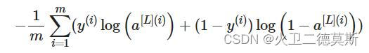

def compute_cost(AL, Y):
    m = Y.shape[1]
    cost = np.dot(Y, np.log(AL.T)) + np.dot(1 - Y, np.log(1 - AL.T))
    cost /= (-m)
    cost = cost.item() # transform [[a]] into a
    return cost

 4 - Backward Propagation

The computation graghic of a 2-layer neural network is as follows:

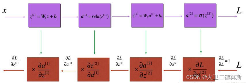
The purple blocks represent the forward propagation, starts from the 1st layer
The red blocks represent the backward propagation, starts from the last(L-th) layer

Observing the rule of chain derivatives, we'll start with calculating dJ/dA[L]=:

For the following loops we'll input da[l], and output dW[l], db[l], dA[l-1], then store them: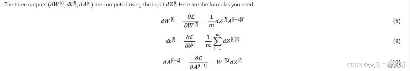

By the way we don't waste to calculate and store dA[0], namely dX, this isn't useful.

def backward(Y, cache, params, backward_functions):
    m = Y.shape[1]
    L = len(backward_functions)

    grads = {}

    Al = cache['A' + str(L)]
    grads['dA' + str(L)] = -(np.divide(Y, Al) - np.divide(1 - Y, 1 - Al))

    for i, backfunc in enumerate(reversed(backward_functions)):
        l = L - i

        dAl = grads['dA' + str(l)]
        Zl = cache['Z' + str(l)]
        # dZl = 0
        if backfunc == relu_backward:
            dZl = relu_backward(dAl, Zl)
        elif backfunc == sigmoid_backward:
            dZl = sigmoid_backward(dAl, Zl)
        elif backfunc == tanh_backward:
            dZl = tanh_backward(dAl, Zl)

        dWl = np.dot(dZl, cache['A' + str(l - 1)].T) / m
        dbl = np.sum(dZl, axis=1, keepdims=True) / m

        # We don't need to cache dA[0], namely dX
        if l != 1:
            dAl_1 = np.dot(params['W' + str(l)].T, dZl)
            grads['dA' + str(l - 1)] = dAl_1
        grads['dW' + str(l)] = dWl
        grads['db' + str(l)] = dbl

    return grads

5 - Update the parameters

def update(params, grads, learning_rate):
    L = int(len(params) / 2)

    for l in range(1, L + 1):
        params['W' + str(l)] -= learning_rate * grads['dW' + str(l)]
        params['b' + str(l)] -= learning_rate * grads['db' + str(l)]

    return params

6 - Deep neural network

def dnn(input_X, Y, nn_structure, forward_functions, learning_rate, num_iterations):
    # generate backward derivative functions according to forward activate functions
    backward_functions = []
    for func in forward_funcs:
        if func == relu:
            backward_functions.append(relu_backward)
        elif func == sigmoid:
            backward_functions.append(sigmoid_backward)
        elif func == tanh:
            backward_functions.append(tanh_backward)

    # Redefine the number of features in nn_structure according to input_X.shape
    nn_structure[0] = input_X.shape[0]
    params = nn_initialize(nn_structure)

    costs = []
    L = len(forward_functions)
    for i in range(num_iterations):
        cache = forward(input_X, params, forward_functions)
        AL = cache['A' + str(L)]
        if i % 10 == 0:
            costs.append(compute_cost(AL, Y))
        grads = backward(Y, cache, params, backward_functions)
        params = update(params, grads, learning_rate)

    return params, costs


def predict(X, params, forward_functions):
    L = len(forward_functions)
    AL = forward(X, params, forward_functions)['A' + str(L)]
    Y_predict = np.round(AL)
    
    return Y_predict

def accuracy(A, Y):
    m = Y.shape[1]
    assert(A.shape == Y.shape)
    acc = (m - np.sum(np.abs(Y - A))) / m
    return acc

 7 - Training/Test dataset

7.1 Cat recognition

We used to conduct this with logistic regression, now try a 2-layer neural network to see if the accuracy is improved.

# Load training and test dataset and process
train_set_x_orig, train_set_y, test_set_x_orig, test_set_y, classes = lr_utils.load_dataset()
train_x_flatten = train_set_x_orig.reshape(train_set_x_orig.shape[0], -1).T
test_x_flatten = test_set_x_orig.reshape(test_set_x_orig.shape[0], -1).T

train_x = train_x_flatten / 255
train_y = train_set_y
test_x = test_x_flatten / 255
test_y = test_set_y

# initialize those hyperparameters for our dnn
layer_dims = [1, 4, 1]  # units on each layer
forward_funcs = [relu, sigmoid]  # activate functions in forward-propagate process
learning_rate = 0.005
num_iteration = 2500

# Run training and prediction
parameters, Costs = dnn(train_x, train_y, layer_dims, forward_funcs, learning_rate, num_iteration)
plt.plot(Costs)
plt.title('Cost function')
plt.xlabel('iteration(×10)')
plt.ylabel('Cost')
plt.show()

Running result:

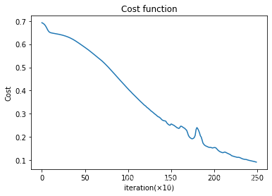
 Let's test the accracies for both training and test datasets

train_y_predict = predict(train_x, parameters, forward_funcs)
test_y_predict = predict(test_x, parameters, forward_funcs)

train_acc = accuracy(train_y_predict, train_y)
test_acc = accuracy(test_y_predict, test_y)
print(f'The training accuracy is:{train_acc*100}%')
print(f'The test accuracy is: {test_acc * 100}%')

The training accuracy is:99.04306220095694%
The test accuracy is: 74.0%

Performance on the test dataset is improved by 4 percent

7.2 Planar classification

7.2.1 Run with a double-sigmoid NN

from planar_utils import plot_decision_boundary, load_planar_dataset


X, Y = load_planar_dataset()
# initialize those hyperparameters for our dnn
layer_dims = [1, 3, 1]  # units on each layer
forward_funcs = [sigmoid, sigmoid]  # activate functions in forward-propagate process
learning_rate = 0.45
num_iteration = 10000

# Run training and prediction
parameters, Costs = dnn(X, Y, layer_dims, forward_funcs, learning_rate, num_iteration)

# Plot the Cost function
plt.subplot(1, 2, 1)
plt.plot(Costs)
plt.title('Cost function')
plt.xlabel('iteration(×10)')
plt.ylabel('Cost')

# Draw the classfication gragh
plt.subplot(1, 2, 2)
plot_decision_boundary(lambda x: predict(x.T, parameters, forward_funcs), X, Y)
plt.show()

y_predict = predict(X, parameters, forward_funcs)
test_acc2 = accuracy(y_predict, Y)
print(f'The training accuracy is: {test_acc2*100}%')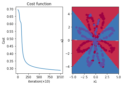

The training accuracy is: 89.5%

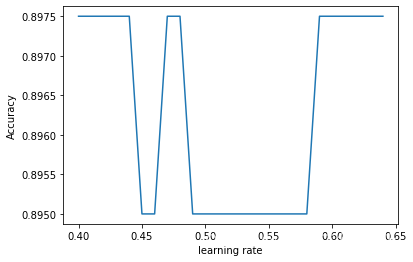
7.2.2 Optimize the hyperparameter α

ACC = []
Learning_rates = np.arange(0.4, 0.65, 0.01)

for lr in Learning_rates:
    parameters, Costs = dnn(X, Y, layer_dims, forward_funcs, lr, num_iteration)
    y_predict = predict(X, parameters, forward_funcs)
    test_acc2 = accuracy(y_predict, Y)
    ACC.append(test_acc2)
    
max_acc = max(ACC)
max_idx = ACC.index(max_acc)
plt.plot(Learning_rates, ACC)
plt.xlabel('learning rate')
plt.ylabel('Accuracy')
print(f'the optimum learning rate is {0.4+0.01*max_idx} with an accuracy of {max_acc*100}%')

the optimum learning rate is 0.4 with an accuracy of 89.75%