一元线性回归代码实现

import matplotlib.pyplot as plt
plt.figure(figsize=(10,4),dpi=80)
x = [[1], [2], [4], [5]]  # 自变量集合为二维结构形式
y = [2, 4, 6, 8]
plt.scatter(x, y)
plt.show()

# 引入Scikit-Learn库快速搭建线性回归模型
from sklearn.linear_model import LinearRegression
regr = LinearRegression()
x = [[1], [2], [4], [5]]
y = [2, 4, 6, 8]
regr.fit(x, y)  # 完成模型搭建
y = regr.predict([[1.5]])
print(y)

x = [[1], [2], [4], [5]]
y = [2, 4, 6, 8]
plt.scatter(x,y)
plt.plot(x, regr.predict(x))  # 预测模型
plt.show()

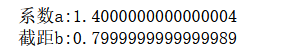
print('系数a:', str(regr.coef_[0]))
print('截距b:', str(regr.intercept_))