2021-01-11

OpenCV—模糊处理与高斯模糊，二值化

模糊处理常用的可以分为三种：
1、均值模糊（均值滤波）
均值滤波是典型的线性滤波算法，它是指在图像上对目标像素给一个模板，该模板包括了其周围的临近像素(以目标像素为中心的周围8个像素，构成一个滤波模板，即去掉目标像素本身)，再用模板中的全体像素的平均值来代替原来像素值。

其缺点也显而易见：

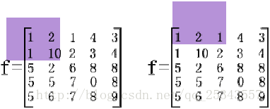
由于图像边框上的像素无法被模板覆盖，所以不做处理。
这当然造成了图像边缘的缺失 。
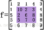
2、中值模糊（滤波）
中值，中间值，将数据从小到大排序后的中间值 ，中值滤波使用一个围绕当前像素的矩形,查找区域内像素的中值,并用该中值替换矩形区域内的其它像素点。
3、高斯模糊
针对图像中的每一个点与高斯内核进行卷积计算,并将计算结果相加,输出到目标图像中。

均值与中值模糊代码

import cv2 as cv
import numpy as np
 
 
def blur_demo(img):
    dst1 = cv.blur(img, (5, 5)) # 均值模糊,（5，5）代表坐标
    cv.imshow("blur_demo", dst1)
 
 
def median_blur_demo(img):
    dst2 = cv.medianBlur(img, 9)  # 中值模糊  有去椒盐的功能（去噪）值得注意的是，ksize的位置必须是整型奇数！
    cv.imshow("medianBlur_demo", dst2)

中值滤波处理椒盐噪声效果显著

自定义模糊

注意要做防止溢出处理

def custom_demo(img):
    kernel = np.ones([5, 5], np.float32)/25
    dst3 = cv.filter2D(img, -1, kernel=kernel)  # 自定义模糊
    cv.imshow("custom_demo", dst3)

自定义锐化操作：

def custom_demo(img):
    # kernel = np.ones([5, 5], np.float32)/25
    kernel = np.array([[1, 1, 1], [1, 1, 1], [1, 1, 1]], np.float32)/9
    dst3 = cv.filter2D(img, -1, kernel=kernel)  # 自定义模糊
    cv.imshow("custom_demo", dst3)

高斯模糊
其在opencv官网的各个参数的说明图

dst = cv2.GaussianBlur(src, ksize, sigmaX, sigmaY)
#ksize,滤波器卷积核的尺寸，必须为元组
#sigmaX：double型，表示高斯核函数在X方向的的标准偏差
#sigmaY：double型，示高斯核函数在Y方向的的标准偏差。若sigmaY为零，就将它设为sigmaX

# 将范围定义在0-255之间
def clamp(pv):
    if pv > 255:
        return 255
    elif pv < 0:
        return 0
    else:return pv
 
 
# 定义高斯噪声函数
def gaussian_demo(img):  #高斯模糊
    h, w, c = img.shape	  #高，宽，通道数
    for row in range(0, h, 1):
        for col in  range(0, w, 1):
            s = np.random.normal(0, 20, 3)
            b = img[row, col, 0]  # blue
            g = img[row, col, 1]  # green![在这里插入图片描述](https://img-blog.csdnimg.cn/20210116211127919.png?x-oss-process=image/watermark,type_ZmFuZ3poZW5naGVpdGk,shadow_10,text_aHR0cHM6Ly9ibG9nLmNzZG4ubmV0L3dlaXhpbl81MjA5MjIyMw==,size_16,color_FFFFFF,t_70)

            r = img[row, col, 2]  # red
            img[row, col, 0] = clamp(b + s[0])
            img[row, col, 1] = clamp(g + s[1])
            img[row, col, 2] = clamp(r + s[2])
    cv.imshow("gaussian_demo", img)

二值化

import cv2

import numpy as np

from matplotlib import pyplot as plt

 

img = cv2.imread('scratch.png', 0)

# global thresholding

ret1, th1 = cv2.threshold(img, 127, 255, cv2.THRESH_BINARY)

# Otsu's thresholding

th2 = cv2.adaptiveThreshold(img, 255, cv2.ADAPTIVE_THRESH_MEAN_C, cv2.THRESH_BINARY, 11, 2)

# Otsu's thresholding

# 阈值一定要设为 0 !

ret3, th3 = cv2.threshold(img, 0, 255, cv2.THRESH_BINARY + cv2.THRESH_OTSU)

# plot all the images and their histograms

images = [img, 0, th1, img, 0, th2, img, 0, th3]

titles = [
'Original Noisy Image', 'Histogram', 'Global Thresholding (v=127)',

  'Original Noisy Image', 'Histogram', "Adaptive Thresholding",

  'Original Noisy Image', 'Histogram', "Otsu's Thresholding"

]

# 这里使用了 pyplot 中画直方图的方法, plt.hist, 要注意的是它的参数是一维数组

# 所以这里使用了( numpy ) ravel 方法,将多维数组转换成一维,也可以使用 flatten 方法

# ndarray.flat 1-D iterator over an array.

# ndarray.flatten 1-D array copy of the elements of an array in row-major order.

for i in range(3):

  plt.subplot(3, 3, i * 3 + 1), plt.imshow(images[i * 3], 'gray')

  plt.title(titles[i * 3]), plt.xticks([]), plt.yticks([])

  plt.subplot(3, 3, i * 3 + 2), plt.hist(images[i * 3].ravel(), 256)

  plt.title(titles[i * 3 + 1]), plt.xticks([]), plt.yticks([])

  plt.subplot(3, 3, i * 3 + 3), plt.imshow(images[i * 3 + 2], 'gray')

  plt.title(titles[i * 3 + 2]), plt.xticks([]), plt.yticks([])

plt.show()

import matplotlib

import matplotlib.pyplot as plt

 

from skimage.data import page

from skimage.filters import (threshold_otsu, threshold_niblack,

               threshold_sauvola)

 

 

matplotlib.rcParams['font.size'] = 9

 

 

image = page()

binary_global = image > threshold_otsu(image)

 

window_size = 25

thresh_niblack = threshold_niblack(image, window_size=window_size, k=0.8)
thresh_sauvola = threshold_sauvola(image, window_size=window_size)

 

binary_niblack = image > thresh_niblack

binary_sauvola = image > thresh_sauvola

 

plt.figure(figsize=(8, 7))

plt.subplot(2, 2, 1)

plt.imshow(image, cmap=plt.cm.gray)

plt.title('Original')

plt.axis('off')

 

plt.subplot(2, 2, 2)

plt.title('Global Threshold')

plt.imshow(binary_global, cmap=plt.cm.gray)

plt.axis('off')

 

plt.subplot(2, 2, 3)

plt.imshow(binary_niblack, cmap=plt.cm.gray)

plt.title('Niblack Threshold')

plt.axis('off')
plt.subplot(2, 2, 4)

plt.imshow(binary_sauvola, cmap=plt.cm.gray)

plt.title('Sauvola Threshold')

plt.axis('off')

 

plt.show()

1. opencv 简单阈值 cv2.threshold

2. opencv 自适应阈值 cv2.adaptiveThreshold (自适应阈值中计算阈值的方法有两种：mean_c 和 guassian_c ，可以尝试用下哪种效果好)

附：现记录几种计算阀值的方法供以后参考

1、双峰法

2、P参数法

3、大津法


4、最大熵阀值法


5、迭代法