scatterpie | ggplot2的几何图形拓展包（1）：如何在地图中添加饼图

前几天有读者在知乎上咨询“散点饼图”的问题，用的是scatterpie工具包，这是ggplot2绘图系统的一个拓展包，一共就包含三个函数：

• geom_scatterpie

• geom_scatterpie_legend

• recenter

下面是geom_scatterpie()函数的语法结构：

geom_scatterpie(
  mapping = NULL,
  data,
  cols,
  pie_scale = 1,
  sorted_by_radius = FALSE,
  legend_name = "type",
  long_format = FALSE,
  ...
)

• cols：绘制饼图的变量名，至少需要两个；

• r：使用在映射函数中的参数，用于指定饼图半径大小。

library(ggplot2)
library(scatterpie)
data.frame(
  x = c(2,4,7,3),
  y = c(1,3,6,4),
  a = 1:4,
  b = 4:1
) -> data
ggplot() +
  geom_scatterpie(aes(x,y), data,
                  cols = c("a","b")) +
  theme_bw()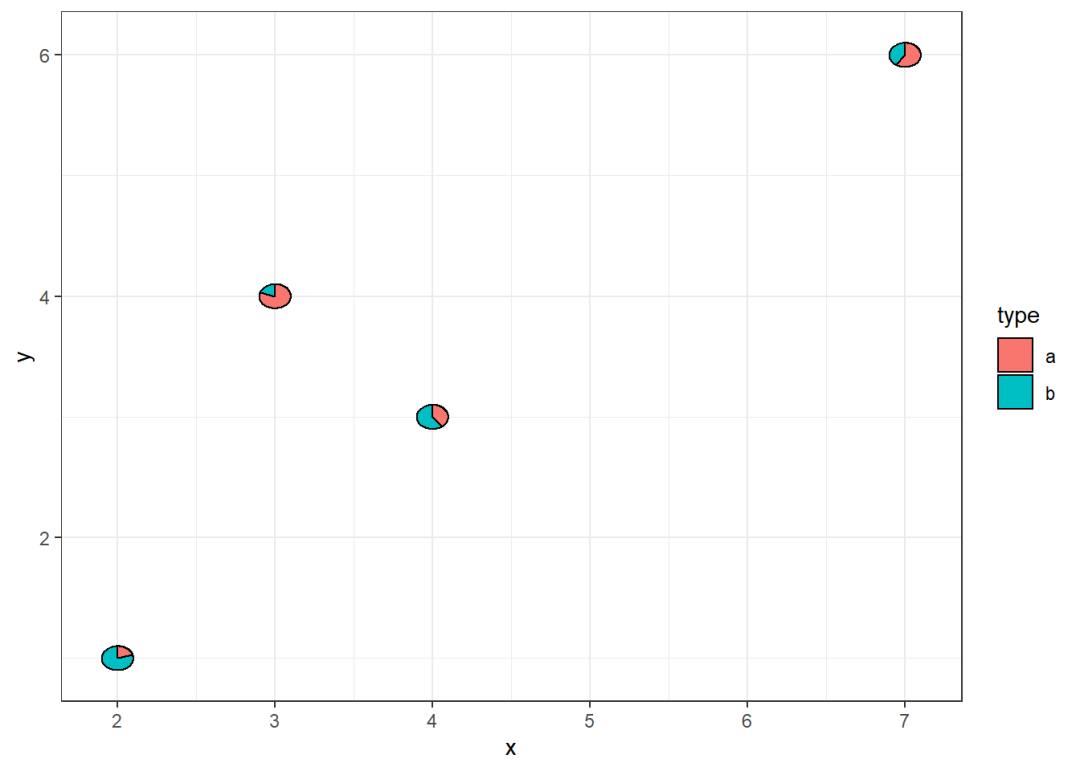

下面这种写法就会报错：

ggplot(data, aes(x,y)) +
  geom_scatterpie(cols = c("a","b")) +
  theme_bw()
# Error in diff(range(data[, xvar])) : 缺少参数"data",也没有缺省值

一般来说，在ggplot2绘图系统中，ggplot()函数指定的是全局参数，几何图形函数没有指定的参数就会自动继承全局的参数，但从上面的报错来看，scatterpie工具包并没有适配这一特点，因此在使用时需要注意。

虽然具有“散点”的特征，但是散点饼图的颜色和形状属性通常不能用于映射，可用的主要是大小属性，也就是半径。

data$r = c(0.2,0.1,0.3,0.4)
ggplot() +
  geom_scatterpie(aes(x ,y,r = r), data,
                  cols = c("a","b"),
                  alpha = 0.5) +
  theme_bw()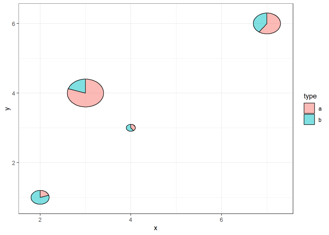

geom_scatterpie_legend()函数可以用来呈现关于半径的图例，完整的语法结构如下：

geom_scatterpie_legend(
  radius,
  x, y,
  n = 5,
  labeller)

• radius：控制半径的变量；该参数同样不能继承自全局；

• x,y：图例放置的横、纵坐标；

• n：呈现的环形个数；

• labeller：半径到标签的映射函数，可缺省。

效果如下：

ggplot() +
  geom_scatterpie(aes(x ,y,r = r), data,
                  cols = c("a","b"),
                  alpha = 0.5) +
  geom_scatterpie_legend(data$r, n = 4,
                         x = 6, y = 2) +
  theme_bw()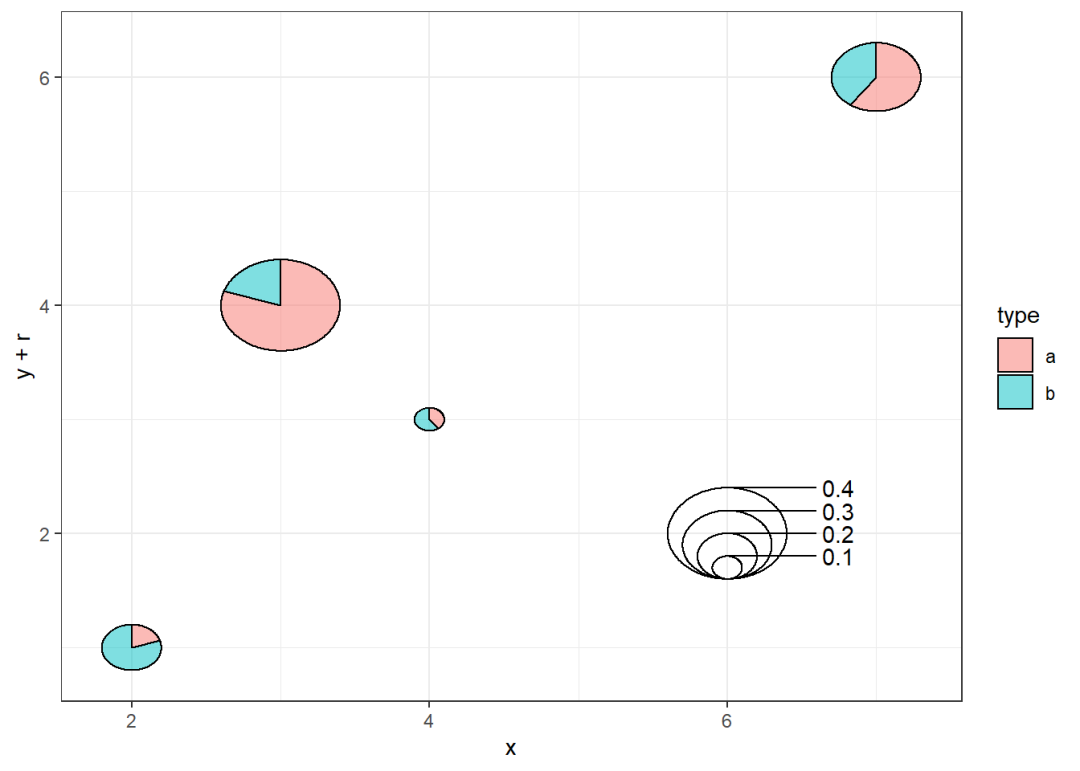

上图中，图例中的半径从内到外依次为0.1、0.2、0.3、0.4，与标签显示的相同，但它实际代表的值可能是10、20、30、40，这时就可以使用labeller参数进行转换。

ggplot() +
  geom_scatterpie(aes(x ,y,r = r), data,
                  cols = c("a","b"),
                  alpha = 0.5) +
  geom_scatterpie_legend(data$r, n = 4,
                         x = 6, y = 2,
                         labeller = function(x) {100*x}) +
  theme_bw()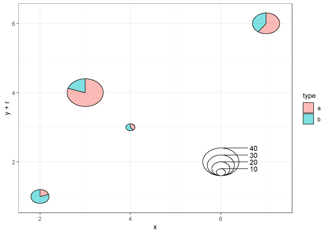

也可以在地图上添加饼图：

library(sf)
China <- read_sf("./China/省.shp")
data.frame(
  A = rpois(35,6),
  B = rpois(35,2),
  C = rpois(35,12),
  lon = st_coordinates(st_centroid(China))[,1],
  lat = st_coordinates(st_centroid(China))[,2]
) -> df

ggplot(China) +
  geom_sf() +
  geom_scatterpie(aes(x = lon, y = lat),
                  data = df,
                  cols = c("A", "B", "C")) +
  theme_bw()

• 这里与前面存在同样一个问题：在绘制地图中，ggplot2原生的函数geom_sf()能够自动识别出空间数据的坐标信息，因此不需要再指定x和y参数，而geom_scatterpie()函数由于不能继承全局参数，数据源、坐标信息等参数都需要单独指定。

总体来说，scatterpie工具包并没有完全地适配ggplot2绘图系统的特点，因此在使用时略显繁琐，但它丰富了几何图形函数的类型还是值得肯定的，希望后续版本能够更加优化。