


专注系列化、高质量的R语言教程
本篇来介绍两种常见的统计检验方法:t检验和F检验。目录如下:
1 t检验
1.1 单样本t检验
1.2 独立样本t检验
1.3 配对样本t检验
1.4 单尾检验
2 F检验
1 t检验
t检验适用于样本量较小、总体方差未知的正态分布的检验。单样本t检验用于检验样本均值是否显著异于给定的总体均值;双样本t检验用于检验两个样本的均值是否存在显著差异,或均值之差是否显著异于给定值,又分为独立样本t检验和配对样本t检验。
R语言中用于t检验的函数是stats工具包中的t.test(),语法结构如下:
t.test(x, y = NULL,
       alternative = c("two.sided", "less", "greater"),
       mu = 0, paired = FALSE, var.equal = FALSE,
       conf.level = 0.95, ...)
1.1 单样本t检验
假设样本来自总体均值为的正态分布,总体方差未知。记样本量为,样本均值为,样本方差为,则如下统计量应服从自由度为的t分布:
若上述假设成立,则统计量应不显著异于0,这也是t检验的零假设;其备选假设是统计量显著异于0,表示不能认为样本来自总体均值为的正态分布。统计检验的显著性水平是错误拒绝零假设(零假设为真、备选假设为假)的概率。
下面代码绘制了自由度为24的t分布的概率密度函数,并以0.05为显著性水平绘制了错误拒绝零假设的区间范围:
par(family = "mono")
x0 <- seq(-5, 5, 0.01)
plot(x0, dt(x0, 24), type = "l",
     yaxs = "i", ylim = c(0,0.45),
     ylab = "p", xlab = "t", las = 1)

t0 <- qt(0.05/2, 24)
x1 <- seq(-5, t0, length.out = 20)
x2 <- seq(-t0, 5, length.out = 20)
segments(x1, 0, x1, dt(x1, 24))
segments(x2, 0, x2, dt(x2, 24))
rm(list = ls())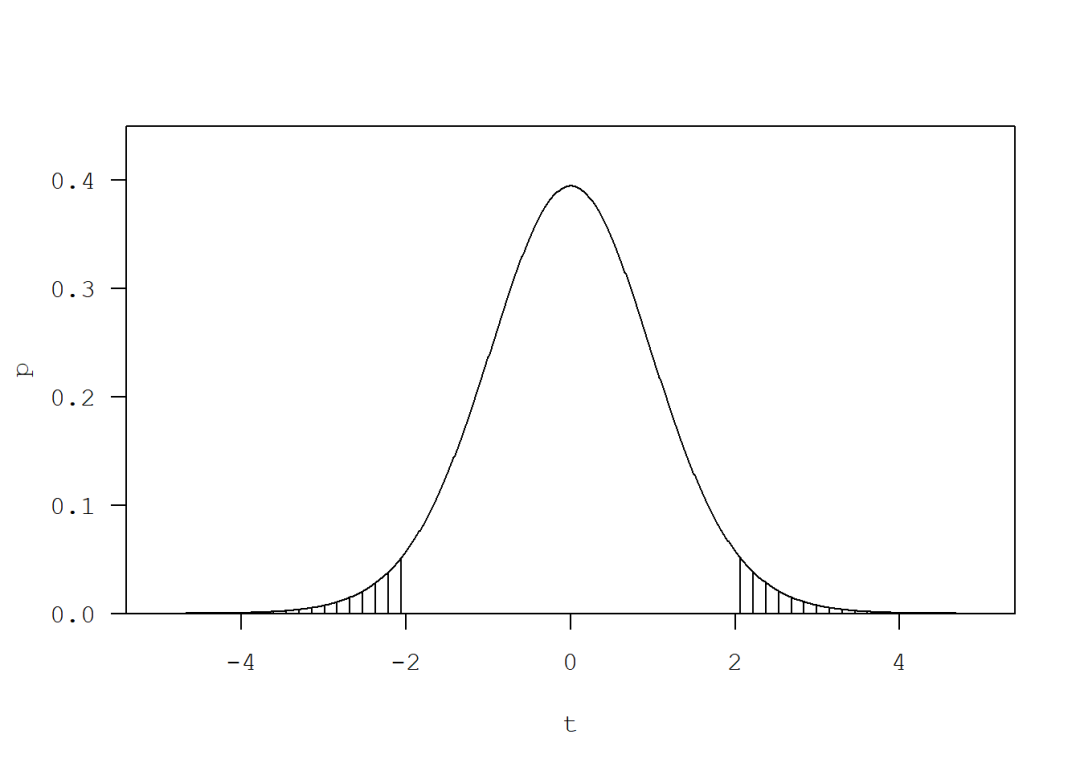
阴影面积之和为显著性水平p;
t分布的概率分布函数沿y轴对称,因此两侧的阴影面积分别为p/2。
生成25个服从均值为5的正态分布的随机数:
set.seed(1107)
x = rnorm(25, 5)
x
##  [1] 5.376401 6.279168 6.006342 5.238824 4.504683 3.906549 5.332404 5.112673
##  [9] 5.211635 5.643550 4.214791 5.890171 5.883895 2.970628 6.363913 4.543970
## [17] 5.547430 3.909453 5.010911 4.746396 4.009331 5.011125 4.809047 4.069485
## [25] 3.738244例1.1:假设该样本来自均值为4的正态分布,若假设成立,则应服从自由度为24的t分布。检验结果如下:
t.test(x, mu = 4)
##  One Sample t-test
##
## data:  x
## t = 5.3635, df = 24, p-value = 1.66e-05
## alternative hypothesis: true mean is not equal to 4
## 95 percent confidence interval:
##  4.574123 5.292358
## sample estimates:
## mean of x
##  4.933241
结果显示统计量为5.3635,置信水平
p-value = 1.66e-05 < 0.05,即错误拒绝零假设的概率很低,因此可以拒绝原假设,也就是不能认为上述统计量服从t分布。
手动计算:
## t统计量
t = (mean(x) - 4)/sqrt(var(x)/length(x))
t
## [1] 5.363467

## 显著性水平
(1 - pt(t, 24))*2
## [1] 1.660442e-05例1.2:假设该样本来自均值为5的正态分布,若假设成立,则应服从自由度为24的t分布。检验结果如下:
t.test(x, mu = 5)
##  One Sample t-test
##
## data:  x
## t = -0.38368, df = 24, p-value = 0.7046
## alternative hypothesis: true mean is not equal to 5
## 95 percent confidence interval:
##  4.574123 5.292358
## sample estimates:
## mean of x
##  4.933241
结果显示统计量为5.3635,置信水平
p-value = 0.7046 > 0.05,即错误拒绝零假设的概率很大,因此不能拒绝原假设,也就是可以认为样本来自均值为5的正态分布。
手动计算:
## t统计量
t2 = (mean(x) - 5)/sqrt(var(x)/length(x))
t2
## [1] -0.3836753

## 显著性水平
pt(t2, 24)*2
## [1] 0.7045971
1.2 独立样本t检验
对于两个来自正态分布的样本,样本均值分别记为、,样本方差分别记为、,样本量分别为、,则如下统计量服从t分布:
若两个样本的均值不存在显著性差异,则统计量应不显著异于0。
例1.3:
set.seed(1107)
x = rnorm(25, 5, sd = 0.1)
y = rnorm(35, 5.2, sd = 0.1)

t.test(x, y)
##  Welch Two Sample t-test
##
## data:  x and y
## t = -9.8654, df = 51.263, p-value = 1.932e-13
## alternative hypothesis: true difference in means is not equal to 0
## 95 percent confidence interval:
##  -0.2684215 -0.1776571
## sample estimates:
## mean of x mean of y
##  4.993324  5.216363
检验结果显示,两个样本的均值存在显著性差异(
p-value = 1.932e-13 < 0.05)。
在进行独立样本t检验之前,通常还应该先使用F检验判断其方差是否具有显著差异:
var.test(x, y)
##  F test to compare two variances
##
## data:  x and y
## F = 1.0378, num df = 24, denom df = 34, p-value = 0.9049
## alternative hypothesis: true ratio of variances is not equal to 1
## 95 percent confidence interval:
##  0.5002457 2.2621714
## sample estimates:
## ratio of variances
##           1.037836
F检验显示,两个样本的方差没有显著性差异,因此应该使用等方差的t检验:
t.test(x, y, var.equal = T)
##  Two Sample t-test
##
## data:  x and y
## t = -9.8965, df = 58, p-value = 4.557e-14
## alternative hypothesis: true difference in means is not equal to 0
## 95 percent confidence interval:
##  -0.2681523 -0.1779263
## sample estimates:
## mean of x mean of y
##  4.993324  5.216363
检验结果显示,两个样本的均值仍然存在显著性差异,并且p值有所下降(
p-value = 4.557e-14 < 1.932e-13)。
1.3 配对样本t检验
假设某样本来自正态分布,其原始序列值为,当前序列值为,二者的序列值存在一一对应关系。记,若相比于,序列值增加了,则如下统计量服从t分布:
例1.4:
set.seed(1107)
x1 = rnorm(25, 5, sd = 0.1)
y1 = x1 + rnorm(25, 0.2, sd = 0.1)

t.test(y1, x1, paired = T, mu = 0.2)
##  Paired t-test
##
## data:  x1 and y1
## t = -25.377, df = 24, p-value < 2.2e-16
## alternative hypothesis: true mean difference is not equal to 0.2
## 95 percent confidence interval:
##  -0.2593173 -0.1902256
## sample estimates:
## mean difference
##      -0.2247714
注意在
t.test()函数中,x1和y1的顺序;检验结果显示,相比于
x1,y1增加的量不显著异于0.2。
1.4 单尾检验
在1.1节的示意图中,我们把错误拒绝零假设的区间范围平均置于概率密度图的两侧,每侧面积各占显著性水平的一半,这种情况称为双尾检验,或双边检验。若把它们置于同一侧,则称为单尾检验,或单边检验;其中全置于左侧,称为左单尾检验;全置于右侧,则称为右单尾检验。
例1.5:
set.seed(1107)
x = rnorm(25, 5)

## 左单尾检验
t.test(x, mu = 4.9, alternative = "less")
##  One Sample t-test
##
## data:  x
## t = 0.19104, df = 24, p-value = 0.5749
## alternative hypothesis: true mean is less than 4.9
## 95 percent confidence interval:
##      -Inf 5.230933
## sample estimates:
## mean of x
##  4.933241

## 右单尾检验
t.test(x, mu = 5.1, alternative = "greater")
##  One Sample t-test
##
## data:  x
## t = -0.95839, df = 24, p-value = 0.8263
## alternative hypothesis: true mean is greater than 5.1
## 95 percent confidence interval:
##  4.635548      Inf
## sample estimates:
## mean of x
##  4.933241
左单尾t检验表明,样本均值不显著小于4.9;右单尾t检验表明,样本均值不显著大于5.1。
t.test(x, mu = 5.1, alternative = "less")
##  One Sample t-test
##
## data:  x
## t = -0.95839, df = 24, p-value = 0.1737
## alternative hypothesis: true mean is less than 5.1
## 95 percent confidence interval:
##      -Inf 5.230933
## sample estimates:
## mean of x
##  4.933241

t.test(x, mu = 4.9, alternative = "greater")
##  One Sample t-test
##
## data:  x
## t = 0.19104, df = 24, p-value = 0.4251
## alternative hypothesis: true mean is greater than 4.9
## 95 percent confidence interval:
##  4.635548      Inf
## sample estimates:
## mean of x
##  4.933241
左单尾t检验表明,样本均值不显著小于5.1;右单尾t检验表明,样本均值不显著大于4.9。
综上,样本均值应不显著异于4.9和5.1,下面的双尾检验也验证了这一点,其95%置信区间为[4.574123, 5.292358]:
t.test(x, mu = 4.9)
##  One Sample t-test
##
## data:  x
## t = 0.19104, df = 24, p-value = 0.8501
## alternative hypothesis: true mean is not equal to 4.9
## 95 percent confidence interval:
##  4.574123 5.292358
## sample estimates:
## mean of x
##  4.933241

t.test(x, mu = 5.1)
##  One Sample t-test
##
## data:  x
## t = -0.95839, df = 24, p-value = 0.3474
## alternative hypothesis: true mean is not equal to 5.1
## 95 percent confidence interval:
##  4.574123 5.292358
## sample estimates:
## mean of x
##  4.933241
2 F检验
对于两个来自正态分布的样本,总体方差分别为、。记样本方差分别为、,样本量分别为、,则如下统计量服从F分布:
若两个样本的总体方差相等,则如下统计量应服从F分布:
R语言中用于F检验的函数是stats工具包中的var.test(),语法结构如下:
var.test(x, y, ratio = 1,
         alternative = c("two.sided", "less", "greater"),
conf.level = 0.95, ...)例2.1:
set.seed(1107)
x <- rnorm(50, mean = 0, sd = 2)
y <- rnorm(30, mean = 1, sd = 1)

var.test(x, y)
##  F test to compare two variances
##
## data:  x and y
## F = 3.4805, num df = 49, denom df = 29, p-value = 0.0005897
## alternative hypothesis: true ratio of variances is not equal to 1
## 95 percent confidence interval:
##  1.748689 6.548289
## sample estimates:
## ratio of variances
##            3.48051
F检验表明,两个样本的方差存在显著区别(
p-value = 0.0005897)。
手动计算:
var(x)/var(y)
## [1] 3.48051例2.2:
set.seed(1107)
x <- rnorm(50, mean = 0, sd = 1)
y <- rnorm(30, mean = 1, sd = 1)

var.test(x, y)
##  F test to compare two variances
##
## data:  x and y
## F = 0.87013, num df = 49, denom df = 29, p-value = 0.6543
## alternative hypothesis: true ratio of variances is not equal to 1
## 95 percent confidence interval:
##  0.4371722 1.6370723
## sample estimates:
## ratio of variances
##          0.8701275
F检验表明,两个样本的方差不存在显著区别(
p-value = 0.6543)。


 1678
1678

 被折叠的 条评论
为什么被折叠?
被折叠的 条评论
为什么被折叠?
 到【灌水乐园】发言


