


1. 特例讲解:解决力扣122题:买卖股票II 力扣
第 1 步:定义状态
状态 dp[i][j] 定义如下:
dp[i][j] 表示到下标为 i 的这一天,持股状态为 j 时,我们手上拥有的最大现金数。
注意:限定持股状态为 j 是为了方便推导状态转移方程,这样的做法满足 无后效性。
其中:
- 第一维 i 表示下标为 i 的那一天( 具有前缀性质,即考虑了之前天数的交易 );
- 第二维 j 表示下标为 i 的那一天是持有股票,还是持有现金。这里 0 表示持有现金(cash),1 表示持有股票(stock)。
第 2 步:思考状态转移方程
- 状态从持有现金(cash)开始,到最后一天我们关心的状态依然是持有现金(cash);
- 每一天状态可以转移,也可以不动。状态转移用下图表示:
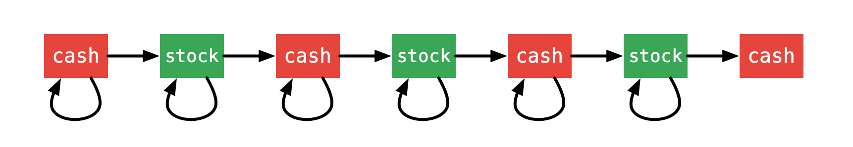
说明:
- 由于不限制交易次数,除了最后一天,每一天的状态可能不变化,也可能转移;
- 写代码的时候,可以不用对最后一天单独处理,输出最后一天,状态为 0 的时候的值即可。
第 3 步:确定初始值
起始时:
- 如果什么都不做,dp[0][0] = 0;
- 如果持有股票,当前拥有的现金数是当天股价的相反数,即 dp[0][1] = -prices[i];
第 4 步:确定输出值
终止的时候,上面也分析了,输出 dp[len - 1][0],因为一定有 dp[len - 1][0] > dp[len - 1][1]。
参考代码如下:
public class Solution {

    public int maxProfit(int[] prices) {
        int len = prices.length;
        if (len < 2) {
            return 0;
        }

        // cash:持有现金
        // hold:持有股票
        // 状态数组
        // 状态转移:cash → hold → cash → hold → cash → hold → cash
        int[] cash = new int[len];
        int[] hold = new int[len];

        cash[0] = 0;
        hold[0] = -prices[0];

        for (int i = 1; i < len; i++) {
            // 这两行调换顺序也是可以的
            cash[i] = Math.max(cash[i - 1], hold[i - 1] + prices[i]);
            hold[i] = Math.max(hold[i - 1], cash[i - 1] - prices[i]);
        }
        return cash[len - 1];
    }
}
考虑优化空间,采用滚动变量替换数组(“滚动数组”技巧。)
public class Solution {

    public int maxProfit(int[] prices) {
        int len = prices.length;
        if (len < 2) {
            return 0;
        }

        // cash:持有现金
        // hold:持有股票
        // 状态转移:cash → hold → cash → hold → cash → hold → cash

        int cash = 0;
        int hold = -prices[0];

        int preCash = cash;
        int preHold = hold;
        for (int i = 1; i < len; i++) {
            cash = Math.max(preCash, preHold + prices[i]);
            hold = Math.max(preHold, preCash - prices[i]);

            preCash = cash;
            preHold = hold;
        }
        return cash;
    }
}
2. 动态规划求解股票系列通解
先牢记,解题关键是 允许的最大交易次数 k 。
具体转自:力扣
符号说明:
- n :表示股票价格数组的长度;
- i: 表示第 i 天(i 的取值范围是 0 到 n - 1);
- k: 表示允许的最大交易次数;
- T[i][k]: 表示在第 i 天结束时,最多进行 k 次交易的情况下可以获得的最大收益。
基准条件:
T[-1][k] = T[i][0] = 0,表示没有进行股票交易时没有收益(注意第一天对应 i = 0,因此 i = -1 表示没有股票交易)。
求解状态转移方程:
第i天可能的操作,共有三种可能:买入、卖出、休息。
题目中存在限制条件,规定不能同时进行多次交易,因此如果决定在第 i 天买入,在买入之前必须持有 0 份股票,如果决定在第 i 天卖出,在卖出之前必须恰好持有 1 份股票。
持有股票的数量是隐藏因素,该因素影响第 i 天可以进行的操作,进而影响最大收益。
因此可对T[i][k] 的定义划分为两项:
-
- T[i][k][0] :在第i天结束时,最多进行k次交易,且在进行操作后持有0份股票的情况下,可获得的最大收益。
- T[i][k][1] :在第i天结束时,最多进行k次交易,且在进行操作后持有1份股票的情况下,可获得的最大收益。
使用新的状态表示之后,可以得到基准情况和状态转移方程。
基准情况:
T[-1][k][0] = 0, T[-1][k][1] = -Infinity
T[i][0][0] = 0, T[i][0][1] = -Infinity
T[-1][k][1] = T[i][0][1] = -Infinity :在没有进行股票交易时不允许持有股票。
状态转移方程:
T[i][k][0] = max(T[i - 1][k][0], T[i - 1][k][1] + prices[i])
T[i][k][1] = max(T[i - 1][k][1], T[i - 1][k - 1][0] - prices[i])
状态转移方程解析:
对于 T[i][k][0] :第 i 天进行的操作只能是休息或卖出,因为在第 i 天结束时持有的股票数量是 0。
T[i - 1][k][0] 是休息操作可得的最大收益,
T[i - 1][k][1] + prices[i] 是卖出操作可得的最大收益。
注意到允许的最大交易次数是不变的,因为每次交易包含两次成对的操作,买入和卖出。只有买入操作会改变允许的最大交易次数。
对于T[i][k][1] : 第 i 天进行的操作只能是休息或买入,因为在第 i 天结束时持有的股票数量是 1。
T[i - 1][k][1] 是休息操作可得的最大收益,
T[i - 1][k - 1][0] - prices[i] 是买入操作可以得到的最大收益。
注意到允许的最大交易次数减少了一次,因为每次买入操作会使用一次交易。
为了得到最后一天结束时的最大收益,可以遍历股票价格数组,根据状态转移方程计算 T[i][k][0] 和 T[i][k][1] 的值。最终答案是 T[n - 1][k][0],因为结束时持有 0 份股票的收益一定大于持有 1 份股票的收益。
应用于特殊情况:
情况一:k = 1
情况一对应的题目是「121. 买卖股票的最佳时机」
对于情况一,每天有两个未知变量:T[i][1][0] 和 T[i][1][1],状态转移方程如下:
T[i][1][0] = max(T[i - 1][1][0], T[i - 1][1][1] + prices[i])
T[i][1][1] = max(T[i - 1][1][1], T[i - 1][0][0] - prices[i]) = max(T[i - 1][1][1], -prices[i])
第二个状态转移方程利用了 T[i][0][0] = 0。
根据上述状态转移方程,可以写出时间复杂度为 O(n) 和空间复杂度为 O(n) 的解法。
class Solution {
    public int maxProfit(int[] prices) {
        if (prices == null || prices.length == 0) {
            return 0;
        }
        int length = prices.length;
        int[][] dp = new int[length][2];
        dp[0][0] = 0;
        dp[0][1] = -prices[0];
        for (int i = 1; i < length; i++) {
            dp[i][0] = Math.max(dp[i - 1][0], dp[i - 1][1] + prices[i]);
            dp[i][1] = Math.max(dp[i - 1][1], -prices[i]);
        }
        return dp[length - 1][0];
    }
}优化空间复杂度为O(1):因为第i天的最大收益只和第i-1天的最大收益有关,故采用滚动变量替代数组
class Solution {
    public int maxProfit(int[] prices) {
        if (prices == null || prices.length == 0) {
            return 0;
        }
        int profit0 = 0, profit1 = -prices[0];
        int length = prices.length;
        for (int i = 1; i < length; i++) {
            profit0 = Math.max(profit0, profit1 + prices[i]);
            profit1 = Math.max(profit1, -prices[i]);
        }
        return profit0;
    }
}
情况二:k 为正无穷
情况二对应的题目是「122. 买卖股票的最佳时机 II」。
如果 k 为正无穷,则 k 和 k - 1 可以看成是相同的,
因此: T[i - 1][k - 1][0] = T[i - 1][k][0] 和 T[i - 1][k - 1][1] = T[i - 1][k][1]。
每天仍有两个未知变量:T[i][k][0] 和 T[i][k][1],其中 k 为正无穷,状态转移方程如下:
T[i][k][0] = max(T[i - 1][k][0], T[i - 1][k][1] + prices[i])
T[i][k][1] = max(T[i - 1][k][1], T[i - 1][k - 1][0] - prices[i]) = max(T[i - 1][k][1], T[i - 1][k][0] - prices[i])
第二个状态转移方程利用了 T[i - 1][k - 1][0] = T[i - 1][k][0]。
根据上述状态转移方程,可以写出时间复杂度为 O(n) 和空间复杂度为 O(n) 的解法。
class Solution {
    public int maxProfit(int[] prices) {
        if (prices == null || prices.length == 0) {
            return 0;
        }
        int length = prices.length;
        int[][] dp = new int[length][2];
        dp[0][0] = 0;
        dp[0][1] = -prices[0];
        for (int i = 1; i < length; i++) {
            dp[i][0] = Math.max(dp[i - 1][0], dp[i - 1][1] + prices[i]);
            dp[i][1] = Math.max(dp[i - 1][1], dp[i - 1][0] - prices[i]);
        }
        return dp[length - 1][0];
    }
}
优化空间复杂度为O(1):
class Solution {
    public int maxProfit(int[] prices) {
        if (prices == null || prices.length == 0) {
            return 0;
        }
        int profit0 = 0, profit1 = -prices[0];
        int length = prices.length;
        for (int i = 1; i < length; i++) {
            int newProfit0 = Math.max(profit0, profit1 + prices[i]);
            int newProfit1 = Math.max(profit1, profit0 - prices[i]);
            profit0 = newProfit0;
            profit1 = newProfit1;
        }
        return profit0;
    }
}
情况三:k = 2
情况三对应的题目是「123. 买卖股票的最佳时机 III」。
情况三和情况一相似,区别之处是,对于情况三,每天有四个未知变量:T[i][1][0]、T[i][1][1]、T[i][2][0]、T[i][2][1],状态转移方程如下:
T[i][2][0] = max(T[i - 1][2][0], T[i - 1][2][1] + prices[i])
T[i][2][1] = max(T[i - 1][2][1], T[i - 1][1][0] - prices[i])
T[i][1][0] = max(T[i - 1][1][0], T[i - 1][1][1] + prices[i])
T[i][1][1] = max(T[i - 1][1][1], T[i - 1][0][0] - prices[i]) = max(T[i - 1][1][1], -prices[i])
第四个状态转移方程利用了 T[i][0][0] = 0。
根据上述状态转移方程,可写出时间复杂度为O(n) 和空间复杂度为 O(n) 的解法。
此处只列出空间复杂度为O(1) 的解法。
class Solution {
    public int maxProfit(int[] prices) {
        if (prices == null || prices.length == 0) {
            return 0;
        }
        int profitOne0 = 0, profitOne1 = -prices[0], profitTwo0 = 0, profitTwo1 = -prices[0];
        int length = prices.length;
        for (int i = 1; i < length; i++) {
            profitTwo0 = Math.max(profitTwo0, profitTwo1 + prices[i]);
            profitTwo1 = Math.max(profitTwo1, profitOne0 - prices[i]);
            profitOne0 = Math.max(profitOne0, profitOne1 + prices[i]);
            profitOne1 = Math.max(profitOne1, -prices[i]);
        }
        return profitTwo0;
    }
}
情况四:k 为任意值
情况四对应的题目是「188. 买卖股票的最佳时机 IV」。
情况四是最通用的情况,对于每一天需要使用不同的 k 值更新所有的最大收益,对应持有 0 份股票或 1 份股票。如果 k 超过一个临界值,最大收益就不再取决于允许的最大交易次数,而是取决于股票价格数组的长度,因此可以进行优化。那么这个临界值是什么呢?
一个有收益的交易至少需要两天(在前一天买入,在后一天卖出,前提是买入价格低于卖出价格)。如果股票价格数组的长度为 n,则有收益的交易的数量最多为 n / 2(整数除法)。因此 k 的临界值是 n / 2。如果给定的 k 不小于临界值,即 k >= n / 2,则可以将 k 扩展为正无穷,此时问题等价于情况二。
根据状态转移方程,可以写出时间复杂度为 O(nk) 和空间复杂度为 O(nk) 的解法。
class Solution {
    public int maxProfit(int k, int[] prices) {
        if (prices == null || prices.length == 0) {
            return 0;
        }
        int length = prices.length;
        if (k >= length / 2) {
            return maxProfit(prices);
        }
        int[][][] dp = new int[length][k + 1][2];
        for (int i = 1; i <= k; i++) {
            dp[0][i][0] = 0;
            dp[0][i][1] = -prices[0];
        }
        for (int i = 1; i < length; i++) {
            for (int j = k; j > 0; j--) {
                dp[i][j][0] = Math.max(dp[i - 1][j][0], dp[i - 1][j][1] + prices[i]);
                dp[i][j][1] = Math.max(dp[i - 1][j][1], dp[i - 1][j - 1][0] - prices[i]);
            }
        }
        return dp[length - 1][k][0];
    }

    public int maxProfit(int[] prices) {
        if (prices == null || prices.length == 0) {
            return 0;
        }
        int length = prices.length;
        int[][] dp = new int[length][2];
        dp[0][0] = 0;
        dp[0][1] = -prices[0];
        for (int i = 1; i < length; i++) {
            dp[i][0] = Math.max(dp[i - 1][0], dp[i - 1][1] + prices[i]);
            dp[i][1] = Math.max(dp[i - 1][1], dp[i - 1][0] - prices[i]);
        }
        return dp[length - 1][0];
    }
}空间复杂度可以降到O(k):
class Solution {
    public int maxProfit(int k, int[] prices) {
        if (prices == null || prices.length == 0) {
            return 0;
        }
        int length = prices.length;
        if (k >= length / 2) {
            return maxProfit(prices);
        }
        int[][] dp = new int[k + 1][2];
        for (int i = 1; i <= k; i++) {
            dp[i][0] = 0;
            dp[i][1] = -prices[0];
        }
        for (int i = 1; i < length; i++) {
            for (int j = k; j > 0; j--) {
                dp[j][0] = Math.max(dp[j][0], dp[j][1] + prices[i]);
                dp[j][1] = Math.max(dp[j][1], dp[j - 1][0] - prices[i]);
            }
        }
        return dp[k][0];
    }

    public int maxProfit(int[] prices) {
        if (prices == null || prices.length == 0) {
            return 0;
        }
        int profit0 = 0, profit1 = -prices[0];
        int length = prices.length;
        for (int i = 1; i < length; i++) {
            int newProfit0 = Math.max(profit0, profit1 + prices[i]);
            int newProfit1 = Math.max(profit1, profit0 - prices[i]);
            profit0 = newProfit0;
            profit1 = newProfit1;
        }
        return profit0;
    }
}
如果不根据 k 的值进行优化,在 k 的值很大的时候会超出时间限制。
对交易次数的循环使用反向循环是为了避免使用临时变量。
情况五:k 为正无穷但有冷却时间
情况五对应的题目是「309. 最佳买卖股票时机含冷冻期」。
由于具有相同的 k 值,因此情况五和情况二非常相似,不同之处在于情况五有「冷却时间」的限制,因此需要对状态转移方程进行一些修改。
在有「冷却时间」的情况下,如果在第 i - 1 天卖出了股票,就不能在第 i 天买入股票。因此,如果要在第 i 天买入股票,第二个状态转移方程中就不能使用 T[i - 1][k][0],而应该使用 T[i - 2][k][0]。
T[i][k][0] = max(T[i - 1][k][0], T[i - 1][k][1] + prices[i])
T[i][k][1] = max(T[i - 1][k][1], T[i - 2][k][0] - prices[i])
列出空间复杂度 O(1) 的解法:
class Solution {
    public int maxProfit(int[] prices) {
        if (prices == null || prices.length == 0) {
            return 0;
        }
        int prevProfit0 = 0, profit0 = 0, profit1 = -prices[0];
        int length = prices.length;
        for (int i = 1; i < length; i++) {
            int nextProfit0 = Math.max(profit0, profit1 + prices[i]);
            int nextProfit1 = Math.max(profit1, prevProfit0 - prices[i]);
            prevProfit0 = profit0;
            profit0 = nextProfit0;
            profit1 = nextProfit1;
        }
        return profit0;
    }
}
情况六:k 为正无穷但有手续费
情况六对应的题目是「714. 买卖股票的最佳时机含手续费」。
由于具有相同的 k 值,因此情况六和情况二非常相似,不同之处在于情况六有「手续费」,因此需要对状态转移方程进行一些修改。
可选择在买入时扣除手续费或卖出时扣除手续费,手续费只需要扣除一次即可。
买入时扣除:
T[i][k][0] = max(T[i - 1][k][0], T[i - 1][k][1] + prices[i])
T[i][k][1] = max(T[i - 1][k][1], T[i - 1][k][0] - prices[i] - fee)
卖出时扣除:
T[i][k][0] = max(T[i - 1][k][0], T[i - 1][k][1] + prices[i] - fee)
T[i][k][1] = max(T[i - 1][k][1], T[i - 1][k][0] - prices[i])
列出空间复杂度为 O(1) 的解法:
class Solution {
    public int maxProfit(int[] prices) {
        if (prices == null || prices.length == 0) {
            return 0;
        }
        int profit0 = 0, profit1 = -prices[0] - fee;
        int length = prices.length;
        for (int i = 1; i < length; i++) {
            int newProfit0 = Math.max(profit0, profit1 + prices[i]);
            int newProfit1 = Math.max(profit1, profit0 - prices[i] - fee);
            profit0 = newProfit0;
            profit1 = newProfit1;
        }
        return profit0;
    }
}
3. 总结
总而言之,股票问题最通用的情况由三个特征决定:当前的天数 i、允许的最大交易次数 k 、每天结束时持有的股票数。


 685
685


 被折叠的 条评论
为什么被折叠?
被折叠的 条评论
为什么被折叠?
 到【灌水乐园】发言


