


决策树是一种基于树状结构的机器学习算法,用于分类和回归任务。它通过一系列的决策节点和分支来对数据进行分类或预测。决策树的生成过程是一个递归的过程,在每个节点上选择最优的特征进行分裂,直到满足某个终止条件为止。
决策树的工作原理可以简述如下:
-
节点选择:从根节点开始,选择最优的特征对数据集进行分割。通常会使用某种指标(例如信息增益、基尼系数等)来评估特征的重要性,选择能够最大程度地提高分类或回归准确度的特征。
-
分裂数据集:根据选择的特征对数据集进行分割,生成新的子节点。分裂的目标是使得各个子节点尽可能地纯净,即同一类别的样本尽可能聚集在一起。
-
递归生成:对每个子节点重复上述过程,直到满足某个停止条件,如达到最大深度、节点中的样本数小于阈值或者特征集为空等。
-
剪枝处理:在生成完整的决策树之后,可以通过剪枝操作来减小决策树的复杂度,防止过拟合。
决策树算法的优点包括易于理解、能够处理离散和连续型数据、对大规模数据集具有较高的效率等。然而,决策树也存在一些缺点,包括容易过拟合、对噪声数据敏感、不稳定性等。因此,在实际应用中,需要根据具体问题的特点选择合适的决策树模型,并进行适当的调参和优化。
ID3
代码:
"""
@实验一:ID3算法
"""
import operator
from math import log
import math
from sklearn.datasets import load_iris
from sklearn.tree import DecisionTreeClassifier, plot_tree
import matplotlib.pyplot as plt
class IDMODEL:
    def __init__(self):

        return None
    '''
    练习一: 计算给定数据集的香农熵
    @:param dataSet 输入的数据集
    pro 类别概率 P(X)
    shannonEnt 数据集类别信息熵  P(X)log2(PX)
    '''
    def calcShannonEnt(self, dataSet):
        numEntries = len(dataSet)
        labelCounts = {}
        for featVec in dataSet:
            currentLabel = featVec[-1]
            if currentLabel not in labelCounts.keys():
                labelCounts[currentLabel] = 0
            else:
                labelCounts[currentLabel] +=1
        shannonEnt = 0.0
        for key in labelCounts:
            prob = float(labelCounts[key])/numEntries
            if prob !=0:

                shannonEnt -=prob * log(prob, 2)

        return shannonEnt

    def splitDataSet(self,dataSet, axis, value):
        retDataSet = []
        for featVec in dataSet:
            if featVec[axis] == value:
                reducedFeatVec = featVec[:axis]
                reducedFeatVec.extend(featVec[axis+1:])
                retDataSet.append(reducedFeatVec)
        return retDataSet

    def chooseBestFeatureToSplit(self, dataSet):
        numFeatures = len(dataSet[0])-1
        baseEntropy = self.calcShannonEnt(dataSet)
        bestInfoGain = 0.0; bestFeature = -1
        for i in range (numFeatures):
            featList = [example[i] for example in dataSet]
            uniqueVals = set(featList)
            newEntropy = 0.0
            for value in uniqueVals:
                subDataSet = self.splitDataSet(dataSet, i, value)
                prob = len(subDataSet)/float(len(dataSet))
                newEntropy +=prob*self.calcShannonEnt(subDataSet)
            infoGain = baseEntropy - newEntropy
            if (infoGain > bestInfoGain):
                bestInfoGain = infoGain
                bestFeature = i
            return bestFeature

    def majorityCnt(self, classList): #少数服从多数
        classCount ={}
        for vote in classList:
            if vote not in classCount.keys():
                classCount[vote] =0
            else:
                classCount[vote] +=1#该类标签下数据个数+1
        sortedClassCount = sorted(classCount.items(), key=operator.itemgetter(1), reverse=True)

        return sortedClassCount[0][0]
    """
    练习三:创建ID3决策树
    @:param dataSet 输入的数据集
    labels 测试属性标签
    classList 创建数据集样本类别列表
    myTree 创建ID3决策树节点保存字典
    :return  myTree
    """
    def createTree(self,dataSet,labels):
        classList = [example[-1] for example in dataSet]#当前数据集的所有标签
        # 若是所有样本属于同一类别,则返回这一类别做节点标记,停止划分
        if classList.count(classList[0])==len(classList):
            return classList[0]
        # 若特征集为空,则返回数据集中样本数最多的类作为节点标记,停止划分
        if len(dataSet[0])==1:
            return self.majorityCnt(classList)#直接投票,返回出现次数最多的标签
        bestFeat = self.chooseBestFeatureToSplit(dataSet)#选择最优测试属性
        bestFeatLabel = labels[bestFeat]#最佳属性的属性名称

        myTree = {bestFeatLabel:{}}#分类结果以字典形式保存
        # 如果最佳划分特征不为空则继续划分
        del(labels[bestFeat]) #在labels数组中删除用来划分的类标签
        featValues = [example[bestFeat] for example in dataSet] #当前数据集中最佳属性的所有属性值
        uniqueVals = set(featValues)#去重得到最佳属性的不同属性值
        for value in uniqueVals:
            subLabels = labels[:]#去除最佳属性后的属性名称列表
            myTree[bestFeatLabel][value]=self.createTree(self.splitDataSet(
                dataSet, bestFeat, value), subLabels)
        return myTree

    def createDataSet(self):
        from sklearn.datasets import load_iris
        iris = load_iris()
        dataSet = iris.data.tolist()
        labels = iris.feature_names

        return dataSet, labels

IDTree = IDMODEL()
dataSet, labels = IDTree.createDataSet()
shannonEnt = IDTree.calcShannonEnt(dataSet)
bestFeature = IDTree.chooseBestFeatureToSplit(dataSet)
myTree=IDTree.createTree(dataSet, labels)
print("======结果分析======")
print("=====数据集DataSet信息熵H(X)=======")
print(shannonEnt)
print("======互信息量最大即条件信息熵最小的测试属性,实现最好的数据集划分方式的测试属性")
print(myTree)
#绘制图形
# 绘制决策树
clf = DecisionTreeClassifier()
iris = load_iris()  # 导入iris数据集
X, y = iris.data, iris.target
clf.fit(X, y)
plt.figure(figsize=(20, 10))
plot_tree(clf, filled=True, feature_names=iris.feature_names)
plt.show() 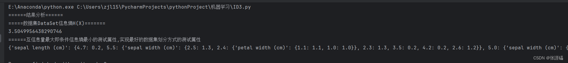

第二种:
import graphviz
from sklearn.datasets import load_iris
from sklearn.model_selection import train_test_split
import numpy as np

# 加载鸢尾花数据集
iris = load_iris()
X = iris.data
y = iris.target

# 合并特征和标签
data = np.column_stack([X, y])

# 将数据集分割为训练集和测试集
X_train, X_test, y_train, y_test = train_test_split(X, y, test_size=0.2, random_state=42)


# 计算信息熵
def entropy(data):
    labels = np.unique(data[:, -1])
    entropy = 0
    for label in labels:
        prob = len(data[data[:, -1] == label]) / len(data)
        entropy -= prob * np.log2(prob)
    print("信息熵为:",entropy)
    return entropy


# 计算条件信息熵
def conditional_entropy(data, attribute_index):
    values = np.unique(data[:, attribute_index])
    conditional_entropy = 0
    for value in values:
        subset = data[data[:, attribute_index] == value]
        prob = len(subset) / len(data)
        conditional_entropy += prob * entropy(subset)
    print("条件信息熵:",conditional_entropy)
    return conditional_entropy


# 根据给定测试属性划分数据集
def split_dataset(data, attribute_index, value):
    return data[data[:, attribute_index] == value]


# 选择最优的测试属性划分数据集
def select_best_attribute(data, attributes):
    best_attribute = None
    min_conditional_entropy = float('inf')
    for attribute_index in attributes:
        temp_conditional_entropy = conditional_entropy(data, attribute_index)
        if temp_conditional_entropy < min_conditional_entropy:
            min_conditional_entropy = temp_conditional_entropy
            best_attribute = attribute_index
    return best_attribute


# 构建决策树的三种情况
# 1. 数据集中的样本属于同一类别
# 2. 属性集为空,无法继续划分
# 3. 已经达到树的最大深度

# 递归建树过程
def build_tree(data, attributes, max_depth):
    # 情况1
    if len(np.unique(data[:, -1])) == 1:
        return data[0, -1]
    # 情况2
    if len(attributes) == 0 or max_depth == 0:
        return np.argmax(np.bincount(data[:, -1].astype(int)))

    # 情况3
    best_attribute = select_best_attribute(data, attributes)
    tree = {best_attribute: {}}
    values = np.unique(data[:, best_attribute])
    new_attributes = [attr for attr in attributes if attr != best_attribute]
    for value in values:
        subset = split_dataset(data, best_attribute, value)
        if len(subset) == 0:
            tree[best_attribute][value] = np.argmax(np.bincount(data[:, -1].astype(int)))
        else:
            tree[best_attribute][value] = build_tree(subset, new_attributes, max_depth - 1)
    return tree


# ID3算法递归建树
def id3(data, max_depth):
    attributes = list(range(data.shape[1] - 1))
    return build_tree(data, attributes, max_depth)


# 分析ID3算法运行结果
def analyze_tree(tree, depth=0):
    if isinstance(tree, dict):
        for key, value in tree.items():
            print('  ' * depth + f'Feature {key}:')
            analyze_tree(value, depth + 1)
    else:
        print('  ' * depth + f'Class Label: {tree}')


# 选择最大深度为3
max_depth = 3

# 运行ID3算法建树
tree = id3(data, max_depth)


# 生成决策树图表
from graphviz import Digraph

def visualize_tree(tree, dot=None):
    if dot is None:
        dot = Digraph()
        dot.attr(rankdir='TB')  # 设置排列方向为从上到下(Top to Bottom)
        dot.attr('node', shape='box')

    if isinstance(tree, dict):
        # 根节点只有一个
        root_key = list(tree.keys())[0]
        dot.node(str(root_key), label=f'Feature {root_key}')

        # 添加根节点到子节点的边
        root_value = tree[root_key]
        if isinstance(root_value, dict):
            for v in root_value:
                dot.edge(str(root_key), str(v), label=str(v))
                visualize_tree(root_value[v], dot)
        else:
            dot.node(str(root_value), label=f'Class Label: {root_value}')
            dot.edge(str(root_key), str(root_value), label=str(root_value))

    return dot

# 示例用法
dot = visualize_tree(tree)
dot.render('stump_tree', format='png', cleanup=True) 

第三种:
from sklearn.datasets import load_iris
from sklearn.tree import DecisionTreeClassifier, plot_tree
from sklearn.model_selection import train_test_split
from sklearn.metrics import accuracy_score
import matplotlib.pyplot as plt
import numpy as np
# 加载数据集
iris = load_iris()
X = iris.data
y = iris.target
# 划分数据集为训练集和测试集
X_train, X_test, y_train, y_test = train_test_split(X, y, test_size=0.2, random_state=42)
# 创建决策树分类器(使用基尼不纯度)
clf = DecisionTreeClassifier(criterion='gini')
# 在训练集上拟合模型
clf.fit(X_train, y_train)
# 在测试集上进行预测
y_pred = clf.predict(X_test)
# 计算准确率
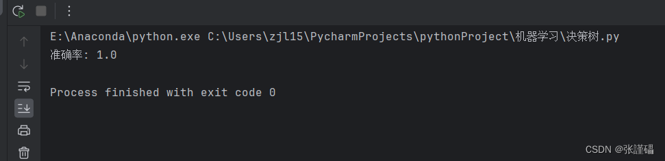
accuracy = accuracy_score(y_test, y_pred)
print("准确率:", accuracy)
# 可视化决策树
plt.figure(figsize=(15, 10))
plot_tree(clf, filled=True, feature_names=iris.feature_names, class_names=iris.target_names)
plt.show()
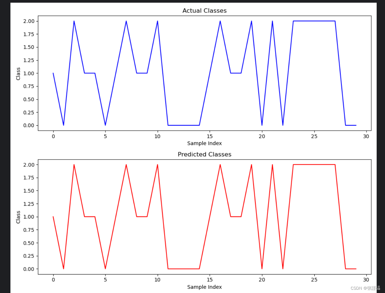
# 创建画布和子图
fig, (ax1, ax2) = plt.subplots(2, 1, figsize=(10, 8))
# 绘制真实值折线图
ax1.plot(np.arange(len(y_test)), y_test, color='blue')
ax1.set_title('Actual Classes')
ax1.set_xlabel('Sample Index')
ax1.set_ylabel('Class')
# 绘制预测值折线图
ax2.plot(np.arange(len(y_test)), y_pred, color='red')
ax2.set_title('Predicted Classes')
ax2.set_xlabel('Sample Index')
ax2.set_ylabel('Class')
# 调整子图之间的间距
plt.tight_layout()
# 显示图表
plt.show()
决策树是一种常用的机器学习算法,可用于分类和回归任务。它通过一系列的决策节点和分支来对数据进行分类或预测。
优点:
- 易于理解和解释:决策树的结构类似于人类的决策过程,因此易于理解和解释,对于非专业人员也较为友好。
- 适用于各种数据类型:决策树可以处理离散型和连续型数据,也不需要对数据进行特征缩放。
- 能够处理大规模数据:相对于其他复杂的算法,决策树在处理大规模数据时具有较高的效率。
- 具有特征选择功能:决策树可以根据特征的重要性进行特征选择,帮助识别最重要的特征。
缺点:
- 容易过拟合:决策树容易过拟合训练数据,特别是当树的深度较大或者分支较多时,容易出现过拟合问题。
- 对数据噪声敏感:决策树对数据中的噪声和异常值比较敏感,可能会影响模型的准确性。
- 不稳定性:数据的小变化可能会导致生成的决策树结构完全不同,因此决策树比较不稳定。
- 可能产生高偏差模型:决策树有时候可能会产生高偏差的模型,特别是当数据关系复杂时,决策树可能无法很好地拟合数据。


 12万+
12万+


 被折叠的 条评论
为什么被折叠?
被折叠的 条评论
为什么被折叠?
 到【灌水乐园】发言


