吴恩达深度学习作业

新图学霸猫

已于 2024-06-08 22:38:38 修改

阅读量159

点赞数 3

文章标签：深度学习人工智能

于 2024-05-11 13:09:27 首次发布

本文链接：https://blog.csdn.net/wenchlove/article/details/138711169

版权

参考资料：吴恩达课后作业
 吴恩达深度学习笔记

课程1 - 神经网络和深度学习

具有神经网络思维的Logistic回归

tips:仅有输入层（12288，1）和输出层（1，1）无隐藏层

import numpy as np
import matplotlib.pyplot as plt
import h5py
import scipy
from PIL import Image
from pandas.core.dtypes.common import classes
from scipy import ndimage
import scipy.misc
from lr_utils import load_dataset

#导入数据集
def init_data():
    train_set_x_orig, train_set_y, test_set_x_orig, test_set_y, classes = load_dataset()
    #看第五章图片
    # index = 5
    # plt.imshow(train_set_x_orig[index])
    # plt.show()
    # print("y = " + str(train_set_y[:, index]) + ", it's a '" + classes[np.squeeze(train_set_y[:, index])].decode(
    #     "utf-8") + "' picture.")

    m_train = train_set_x_orig.shape[0]  # 训练集里图片的数量。
    m_test = test_set_x_orig.shape[0]  # 测试集里图片的数量。
    num_px = train_set_x_orig.shape[1]  # 训练集里图片的宽度
    num_py = train_set_x_orig.shape[2]  # 训练集里图片的宽度

    #看一看 加载的东西的具体情况
    # print("Number of training examples:m_train = "+str(m_train))
    # print("Number of testing examples:m_test = "+str(m_test))
    # print ("Height of each image: num_px = " + str(num_px))
    # print("Each image is of size: (" + str(num_px) + ", " + str(num_py) + ", 3)")
    #
    # print("train_set_x shape: " + str(train_set_x_orig.shape))
    # print("train_set_y shape: " + str(train_set_y.shape))
    #
    # print("test_set_x shape: " + str(test_set_x_orig.shape))
    # print("test_set_y shape: " + str(test_set_y.shape))

    # X_flatten = X.reshape(X.shape [0]，-1).T ＃X.T是X的转置
    # 将训练集的维度降低并转置。
    train_set_x_flatten = train_set_x_orig.reshape(train_set_x_orig.shape[0], -1).T
    # 将测试集的维度降低并转置。
    test_set_x_flatten = test_set_x_orig.reshape(test_set_x_orig.shape[0], -1).T

    # 看看降维之后的情况是怎么样的
    # print("训练集降维最后的维度: " + str(train_set_x_flatten.shape))
    # print("训练集_标签的维数: " + str(train_set_y.shape))
    # print("测试集降维之后的维度: " + str(test_set_x_flatten.shape))
    # print("测试集_标签的维数: " + str(test_set_y.shape))

    train_set_x = train_set_x_flatten / 255
    test_set_x = test_set_x_flatten / 255
    return (train_set_x, train_set_y, test_set_x, test_set_y)

def sigmoid(x):
    s=1/(1+np.exp(-x))
    return s

def initialize_with_zeros(dim):
    w=np.zeros((dim,1))
    b=0
    assert (w.shape==(dim,1))
    assert (isinstance(b,float) or isinstance(b,int))
    return w,b

def propagate(w,b,X,Y):
       m=X.shape[1]
       #正向传播
       Z=np.dot(w.T,X)+b
       A=sigmoid(Z)
       #计算J
       cost=-1/m*np.sum(Y*np.log(A)+(1-Y)*np.log(1-A))

       #反向传播
       dw=1/m*np.dot(X,(A-Y).T)
       db=1/m*np.sum(A-Y)

       assert (dw.shape==w.shape)
       assert (db.dtype==float)
       cost=np.squeeze(cost)
       assert (cost.shape==())

       grads={"dw":dw,"db":db}
       return grads,cost

def optimize(w,b,X,Y,num_iterations,learning_rate,print_cost):
    costs=[]
    for i in range(num_iterations):
        grads,cost=propagate(w,b,X,Y)
        dw=grads["dw"]
        db=grads["db"]

        w=w-learning_rate*dw
        b=b-learning_rate*db

        #每100次记录一次cost
        if i%100==0:
            costs.append(cost)

        if print_cost and i%100==0:
            print("Cost after iteration %i: %f" % (i, cost))

        params={"w":w,"b":b}
        grads={"dw":dw,"db":db}

    return params,grads,costs

def predict(w,b,X):
    m=X.shape[1]
    Y_prediction=np.zeros((1,m))
    w=w.reshape(X.shape[0],1)

    Z=np.dot(w.T,X)+b
    A=sigmoid(Z)

    for i in range(A.shape[1]):
        if(A[0,i]<=0.5):
            Y_prediction[0,i]=0
        else :
            Y_prediction[0, i] = 1

    assert(Y_prediction.shape == (1,m))
    return Y_prediction

def model(X_train,Y_train,X_test,Y_test,num_iterations,learning_rate,print_cost):
    #初始化参数
    w,b=initialize_with_zeros(X_train.shape[0])
    #梯度下降
    parameters,grads,costs=optimize(w,b,X_train,Y_train,num_iterations,learning_rate,print_cost)
    w=parameters["w"]
    b=parameters["b"]
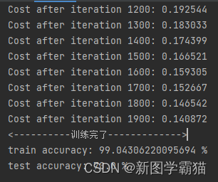
    print("<----------训练完了------------->")
    # 预测测试/训练集的例子
    Y_prediction_test = predict(w, b, X_test)
    Y_prediction_train = predict(w, b, X_train)
    # 打印训练后的准确性
    print("train accuracy: {} %".format(100 - np.mean(np.abs(Y_prediction_train - Y_train)) * 100))
    print("test accuracy: {} %".format(100 - np.mean(np.abs(Y_prediction_test - Y_test)) * 100))
    d = {"costs": costs,
         "Y_prediction_test": Y_prediction_test,
         "Y_prediction_train": Y_prediction_train,
         "w": w,
         "b": b,
         "learning_rate": learning_rate,
         "num_iterations": num_iterations}

    return d


if __name__=="__main__":
    train_set_x, train_set_y, test_set_x, test_set_y = init_data()
    print("====================测试model====================")
    # 这里加载的是真实的数据
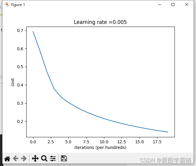
    d = model(train_set_x, train_set_y, test_set_x, test_set_y, num_iterations=2000, learning_rate=0.005,print_cost=True)


    costs = np.squeeze(d['costs'])
    plt.plot(costs)
    plt.ylabel('cost')
    plt.xlabel('iterations (per hundreds)')
    plt.title("Learning rate =" + str(d["learning_rate"]))
    plt.show()

在这里插入图片描述

一层隐藏层的神经网络分类二维数据

practice.py

# -*- coding: utf-8 -*-

import numpy as np
import matplotlib.pyplot as plt
from testCases import *
import sklearn
import sklearn.datasets
import sklearn.linear_model
from planar_utils import plot_decision_boundary, sigmoid, load_planar_dataset, load_extra_datasets

#%matplotlib inline #如果你使用用的是Jupyter Notebook的话请取消注释。

np.random.seed(1) #设置一个固定的随机种子，以保证接下来的步骤中我们的结果是一致的。

X, Y = load_planar_dataset()
#plt.scatter(X[0, :], X[1, :], c=Y, s=40, cmap=plt.cm.Spectral) #绘制散点图
shape_X = X.shape
shape_Y = Y.shape
m = Y.shape[1]  # 训练集里面的数量

print ("X的维度为: " + str(shape_X))
print ("Y的维度为: " + str(shape_Y))
print ("数据集里面的数据有：" + str(m) + " 个")

def layer_sizes(X , Y):
    """
    参数：
     X - 输入数据集,维度为（输入的数量，训练/测试的数量）
     Y - 标签，维度为（输出的数量，训练/测试数量）

    返回：
     n_x - 输入层的数量
     n_h - 隐藏层的数量
     n_y - 输出层的数量
    """
    n_x = X.shape[0] #输入层
    n_h = 4 #，隐藏层，硬编码为4
    n_y = Y.shape[0] #输出层

    return (n_x,n_h,n_y)

def initialize_parameters( n_x , n_h ,n_y):
    """
    参数：
        n_x - 输入节点的数量
        n_h - 隐藏层节点的数量
        n_y - 输出层节点的数量

    返回：
        parameters - 包含参数的字典：
            W1 - 权重矩阵,维度为（n_h，n_x）
            b1 - 偏向量，维度为（n_h，1）
            W2 - 权重矩阵，维度为（n_y，n_h）
            b2 - 偏向量，维度为（n_y，1）

    """
    np.random.seed(2) #指定一个随机种子，以便你的输出与我们的一样。
    W1 = np.random.randn(n_h,n_x) * 0.01
    b1 = np.zeros(shape=(n_h, 1))
    W2 = np.random.randn(n_y,n_h) * 0.01
    b2 = np.zeros(shape=(n_y, 1))

    #使用断言确保我的数据格式是正确的
    assert(W1.shape == ( n_h , n_x ))
    assert(b1.shape == ( n_h , 1 ))
    assert(W2.shape == ( n_y , n_h ))
    assert(b2.shape == ( n_y , 1 ))

    parameters = {"W1" : W1,
                  "b1" : b1,
                  "W2" : W2,
                  "b2" : b2 }

    return parameters

def forward_propagation( X , parameters ):
    """
    参数：
         X - 维度为（n_x，m）的输入数据。
         parameters - 初始化函数（initialize_parameters）的输出

    返回：
         A2 - 使用sigmoid()函数计算的第二次激活后的数值
         cache - 包含“Z1”，“A1”，“Z2”和“A2”的字典类型变量
     """
    W1 = parameters["W1"]
    b1 = parameters["b1"]
    W2 = parameters["W2"]
    b2 = parameters["b2"]
    #前向传播计算A2
    Z1 = np.dot(W1 , X) + b1
    A1 = np.tanh(Z1)
    Z2 = np.dot(W2 , A1) + b2
    A2 = sigmoid(Z2)
    #使用断言确保我的数据格式是正确的
    assert(A2.shape == (1,X.shape[1]))
    cache = {"Z1": Z1,
             "A1": A1,
             "Z2": Z2,
             "A2": A2}

    return (A2, cache)

def compute_cost(A2,Y,parameters):
    """
    计算方程（6）中给出的交叉熵成本，

    参数：
         A2 - 使用sigmoid()函数计算的第二次激活后的数值
         Y - "True"标签向量,维度为（1，数量）
         parameters - 一个包含W1，B1，W2和B2的字典类型的变量

    返回：
         成本 - 交叉熵成本给出方程（13）
    """

    m = Y.shape[1]
    W1 = parameters["W1"]
    W2 = parameters["W2"]

    #计算成本
    logprobs = logprobs = np.multiply(np.log(A2), Y) + np.multiply((1 - Y), np.log(1 - A2))
    cost = - np.sum(logprobs) / m
    cost = float(np.squeeze(cost))

    assert(isinstance(cost,float))

    return cost

def backward_propagation(parameters,cache,X,Y):
    """
    使用上述说明搭建反向传播函数。

    参数：
     parameters - 包含我们的参数的一个字典类型的变量。
     cache - 包含“Z1”，“A1”，“Z2”和“A2”的字典类型的变量。
     X - 输入数据，维度为（2，数量）
     Y - “True”标签，维度为（1，数量）

    返回：
     grads - 包含W和b的导数一个字典类型的变量。
    """
    m = X.shape[1]

    W1 = parameters["W1"]
    W2 = parameters["W2"]

    A1 = cache["A1"]
    A2 = cache["A2"]

    dZ2= A2 - Y
    dW2 = (1 / m) * np.dot(dZ2, A1.T)
    db2 = (1 / m) * np.sum(dZ2, axis=1, keepdims=True)
    dZ1 = np.multiply(np.dot(W2.T, dZ2), 1 - np.power(A1, 2))
    dW1 = (1 / m) * np.dot(dZ1, X.T)
    db1 = (1 / m) * np.sum(dZ1, axis=1, keepdims=True)
    grads = {"dW1": dW1,
             "db1": db1,
             "dW2": dW2,
             "db2": db2 }

    return grads

def update_parameters(parameters,grads,learning_rate=1.2):
    """
    使用上面给出的梯度下降更新规则更新参数

    参数：
     parameters - 包含参数的字典类型的变量。
     grads - 包含导数值的字典类型的变量。
     learning_rate - 学习速率

    返回：
     parameters - 包含更新参数的字典类型的变量。
    """
    W1,W2 = parameters["W1"],parameters["W2"]
    b1,b2 = parameters["b1"],parameters["b2"]

    dW1,dW2 = grads["dW1"],grads["dW2"]
    db1,db2 = grads["db1"],grads["db2"]

    W1 = W1 - learning_rate * dW1
    b1 = b1 - learning_rate * db1
    W2 = W2 - learning_rate * dW2
    b2 = b2 - learning_rate * db2

    parameters = {"W1": W1,
                  "b1": b1,
                  "W2": W2,
                  "b2": b2}

    return parameters

def nn_model(X,Y,n_h,num_iterations,print_cost=False):
    """
    参数：
        X - 数据集,维度为（2，示例数）
        Y - 标签，维度为（1，示例数）
        n_h - 隐藏层的数量
        num_iterations - 梯度下降循环中的迭代次数
        print_cost - 如果为True，则每1000次迭代打印一次成本数值

    返回：
        parameters - 模型学习的参数，它们可以用来进行预测。
     """

    np.random.seed(3) #指定随机种子
    n_x = layer_sizes(X, Y)[0]
    n_y = layer_sizes(X, Y)[2]

    parameters = initialize_parameters(n_x,n_h,n_y)
    W1 = parameters["W1"]
    b1 = parameters["b1"]
    W2 = parameters["W2"]
    b2 = parameters["b2"]

    for i in range(num_iterations):
        A2 , cache = forward_propagation(X,parameters)
        cost = compute_cost(A2,Y,parameters)
        grads = backward_propagation(parameters,cache,X,Y)
        parameters = update_parameters(parameters,grads,learning_rate = 0.5)

        if print_cost:
            if i%1000 == 0:
                print("第 ",i," 次循环，成本为："+str(cost))
    return parameters

def predict(parameters,X):
    """
    使用学习的参数，为X中的每个示例预测一个类

    参数：
        parameters - 包含参数的字典类型的变量。
        X - 输入数据（n_x，m）

    返回
        predictions - 我们模型预测的向量（红色：0 /蓝色：1）

     """
    A2 , cache = forward_propagation(X,parameters)
    predictions = np.round(A2)

    return predictions

parameters = nn_model(X, Y, n_h = 4, num_iterations=10000, print_cost=True)

#绘制边界
plot_decision_boundary(lambda x: predict(parameters, x.T), X, Y)
plt.title("Decision Boundary for hidden layer size " + str(4))

predictions = predict(parameters, X)
accuracy = (np.dot(Y, predictions.T).item() + np.dot(1 - Y, 1 - predictions.T).item()) / float(Y.size) * 100
print('准确率: %d%%' % accuracy)
#print ('准确率: %d' % float((np.dot(Y, predictions.T) + np.dot(1 - Y, 1 - predictions.T)) / float(Y.size) * 100) + '%')

"""
plt.figure(figsize=(16, 32))
hidden_layer_sizes = [1, 2, 3, 4, 5, 20, 50] #隐藏层数量
for i, n_h in enumerate(hidden_layer_sizes):
    plt.subplot(5, 2, i + 1)
    plt.title('Hidden Layer of size %d' % n_h)
    parameters = nn_model(X, Y, n_h, num_iterations=5000)
    plot_decision_boundary(lambda x: predict(parameters, x.T), X, Y)
    predictions = predict(parameters, X)
    accuracy = float((np.dot(Y, predictions.T) + np.dot(1 - Y, 1 - predictions.T)) / float(Y.size) * 100)
    print ("隐藏层的节点数量： {}  ，准确率: {} %".format(n_h, accuracy))
"""

testCases.py

#-*- coding: UTF-8 -*-

import numpy as np

def layer_sizes_test_case():
    np.random.seed(1)
    X_assess = np.random.randn(5, 3)
    Y_assess = np.random.randn(2, 3)
    return X_assess, Y_assess

def initialize_parameters_test_case():
    n_x, n_h, n_y = 2, 4, 1
    return n_x, n_h, n_y

def forward_propagation_test_case():
    np.random.seed(1)
    X_assess = np.random.randn(2, 3)

    parameters = {'W1': np.array([[-0.00416758, -0.00056267],
        [-0.02136196,  0.01640271],
        [-0.01793436, -0.00841747],
        [ 0.00502881, -0.01245288]]),
     'W2': np.array([[-0.01057952, -0.00909008,  0.00551454,  0.02292208]]),
     'b1': np.array([[ 0.],
        [ 0.],
        [ 0.],
        [ 0.]]),
     'b2': np.array([[ 0.]])}

    return X_assess, parameters

def compute_cost_test_case():
    np.random.seed(1)
    Y_assess = np.random.randn(1, 3)
    parameters = {'W1': np.array([[-0.00416758, -0.00056267],
        [-0.02136196,  0.01640271],
        [-0.01793436, -0.00841747],
        [ 0.00502881, -0.01245288]]),
     'W2': np.array([[-0.01057952, -0.00909008,  0.00551454,  0.02292208]]),
     'b1': np.array([[ 0.],
        [ 0.],
        [ 0.],
        [ 0.]]),
     'b2': np.array([[ 0.]])}

    a2 = (np.array([[ 0.5002307 ,  0.49985831,  0.50023963]]))

    return a2, Y_assess, parameters

def backward_propagation_test_case():
    np.random.seed(1)
    X_assess = np.random.randn(2, 3)
    Y_assess = np.random.randn(1, 3)
    parameters = {'W1': np.array([[-0.00416758, -0.00056267],
        [-0.02136196,  0.01640271],
        [-0.01793436, -0.00841747],
        [ 0.00502881, -0.01245288]]),
     'W2': np.array([[-0.01057952, -0.00909008,  0.00551454,  0.02292208]]),
     'b1': np.array([[ 0.],
        [ 0.],
        [ 0.],
        [ 0.]]),
     'b2': np.array([[ 0.]])}

    cache = {'A1': np.array([[-0.00616578,  0.0020626 ,  0.00349619],
         [-0.05225116,  0.02725659, -0.02646251],
         [-0.02009721,  0.0036869 ,  0.02883756],
         [ 0.02152675, -0.01385234,  0.02599885]]),
  'A2': np.array([[ 0.5002307 ,  0.49985831,  0.50023963]]),
  'Z1': np.array([[-0.00616586,  0.0020626 ,  0.0034962 ],
         [-0.05229879,  0.02726335, -0.02646869],
         [-0.02009991,  0.00368692,  0.02884556],
         [ 0.02153007, -0.01385322,  0.02600471]]),
  'Z2': np.array([[ 0.00092281, -0.00056678,  0.00095853]])}
    return parameters, cache, X_assess, Y_assess

def update_parameters_test_case():
    parameters = {'W1': np.array([[-0.00615039,  0.0169021 ],
        [-0.02311792,  0.03137121],
        [-0.0169217 , -0.01752545],
        [ 0.00935436, -0.05018221]]),
 'W2': np.array([[-0.0104319 , -0.04019007,  0.01607211,  0.04440255]]),
 'b1': np.array([[ -8.97523455e-07],
        [  8.15562092e-06],
        [  6.04810633e-07],
        [ -2.54560700e-06]]),
 'b2': np.array([[  9.14954378e-05]])}

    grads = {'dW1': np.array([[ 0.00023322, -0.00205423],
        [ 0.00082222, -0.00700776],
        [-0.00031831,  0.0028636 ],
        [-0.00092857,  0.00809933]]),
 'dW2': np.array([[ -1.75740039e-05,   3.70231337e-03,  -1.25683095e-03,
          -2.55715317e-03]]),
 'db1': np.array([[  1.05570087e-07],
        [ -3.81814487e-06],
        [ -1.90155145e-07],
        [  5.46467802e-07]]),
 'db2': np.array([[ -1.08923140e-05]])}
    return parameters, grads

def nn_model_test_case():
    np.random.seed(1)
    X_assess = np.random.randn(2, 3)
    Y_assess = np.random.randn(1, 3)
    return X_assess, Y_assess

def predict_test_case():
    np.random.seed(1)
    X_assess = np.random.randn(2, 3)
    parameters = {'W1': np.array([[-0.00615039,  0.0169021 ],
        [-0.02311792,  0.03137121],
        [-0.0169217 , -0.01752545],
        [ 0.00935436, -0.05018221]]),
     'W2': np.array([[-0.0104319 , -0.04019007,  0.01607211,  0.04440255]]),
     'b1': np.array([[ -8.97523455e-07],
        [  8.15562092e-06],
        [  6.04810633e-07],
        [ -2.54560700e-06]]),
     'b2': np.array([[  9.14954378e-05]])}
    return parameters, X_assess

planar_utils.py

import matplotlib.pyplot as plt
import numpy as np
import sklearn
import sklearn.datasets
import sklearn.linear_model

def plot_decision_boundary(model, X, y):
    # Set min and max values and give it some padding
    x_min, x_max = X[0, :].min() - 1, X[0, :].max() + 1
    y_min, y_max = X[1, :].min() - 1, X[1, :].max() + 1
    h = 0.01
    # Generate a grid of points with distance h between them
    xx, yy = np.meshgrid(np.arange(x_min, x_max, h), np.arange(y_min, y_max, h))
    # Predict the function value for the whole grid
    Z = model(np.c_[xx.ravel(), yy.ravel()])
    Z = Z.reshape(xx.shape)
    # Plot the contour and training examples
    plt.contourf(xx, yy, Z, cmap=plt.cm.Spectral)
    plt.ylabel('x2')
    plt.xlabel('x1')
    plt.scatter(X[0, :], X[1, :], c=np.squeeze(y), cmap=plt.cm.Spectral)


def sigmoid(x):
    s = 1/(1+np.exp(-x))
    return s

def load_planar_dataset():
    np.random.seed(1)
    m = 400 # number of examples
    N = int(m/2) # number of points per class
    D = 2 # dimensionality
    X = np.zeros((m,D)) # data matrix where each row is a single example
    Y = np.zeros((m,1), dtype='uint8') # labels vector (0 for red, 1 for blue)
    a = 4 # maximum ray of the flower

    for j in range(2):
        ix = range(N*j,N*(j+1))
        t = np.linspace(j*3.12,(j+1)*3.12,N) + np.random.randn(N)*0.2 # theta
        r = a*np.sin(4*t) + np.random.randn(N)*0.2 # radius
        X[ix] = np.c_[r*np.sin(t), r*np.cos(t)]
        Y[ix] = j

    X = X.T
    Y = Y.T

    return X, Y

def load_extra_datasets():
    N = 200
    noisy_circles = sklearn.datasets.make_circles(n_samples=N, factor=.5, noise=.3)
    noisy_moons = sklearn.datasets.make_moons(n_samples=N, noise=.2)
    blobs = sklearn.datasets.make_blobs(n_samples=N, random_state=5, n_features=2, centers=6)
    gaussian_quantiles = sklearn.datasets.make_gaussian_quantiles(mean=None, cov=0.5, n_samples=N, n_features=2, n_classes=2, shuffle=True, random_state=None)
    no_structure = np.random.rand(N, 2), np.random.rand(N, 2)

    return noisy_circles, noisy_moons, blobs, gaussian_quantiles, no_structure

具有L层的神经网络

import numpy as np
import h5py
import matplotlib.pyplot as plt
from testCases import *
from dnn_utils import sigmoid, sigmoid_backward, relu, relu_backward
import lr_utils


np.random.seed(1)

def initialize_parameters(n_x, n_h, n_y):

    W1 = np.random.randn(n_h, n_x) * 0.01
    b1 = np.zeros((n_h, 1))
    W2 = np.random.randn(n_y, n_h) * 0.01
    b2 = np.zeros((n_y, 1))

    # 使用断言确保我的数据格式是正确的
    assert (W1.shape == (n_h, n_x))
    assert (b1.shape == (n_h, 1))
    assert (W2.shape == (n_y, n_h))
    assert (b2.shape == (n_y, 1))

    parameters = {"W1": W1,
                  "b1": b1,
                  "W2": W2,
                  "b2": b2}

    return parameters


#初始化网络参数
def initialize_parameters_deep(layer_dims):

    np.random.seed(3)
    parameters = {}
    L = len(layer_dims)  # 网络层数

    for l in range(1, L):
        parameters['W' + str(l)] = np.random.randn(layer_dims[l], layer_dims[l - 1]) / np.sqrt(layer_dims[l - 1])
        parameters['b' + str(l)] = np.zeros((layer_dims[l], 1))

        # 确保我要的数据的格式是正确的
        assert (parameters['W' + str(l)].shape == (layer_dims[l], layer_dims[l - 1]))
        assert (parameters['b' + str(l)].shape == (layer_dims[l], 1))

    return parameters

#前向传播 线性传播
def linear_forward(A, W, b):

    Z = np.dot(W, A) + b

    assert (Z.shape == (W.shape[0], A.shape[1]))
    cache = (A, W, b)

    return Z, cache

#前向传播 线性激活
def linear_activation_forward(A_prev, W, b, activation):

    if activation == "sigmoid":
        Z, linear_cache = linear_forward(A_prev, W, b)
        A, activation_cache = sigmoid(Z)

    elif activation == "relu":
        Z, linear_cache = linear_forward(A_prev, W, b)
        A, activation_cache = relu(Z)

    assert (A.shape == (W.shape[0], A_prev.shape[1]))
    cache = (linear_cache, activation_cache)

    return A, cache

#L层神经网络的前向传播
def L_model_forward(X, parameters):

    caches = []
    A = X
    L = len(parameters) // 2  # 神经网络的层数

    for l in range(1, L):
        A_prev = A
        A, cache = linear_activation_forward(A_prev, parameters['W' + str(l)], parameters['b' + str(l)],
                                             activation="relu")
        caches.append(cache)

    AL, cache = linear_activation_forward(A, parameters['W' + str(L)], parameters['b' + str(L)], activation="sigmoid")
    caches.append(cache)

    assert (AL.shape == (1, X.shape[1]))

    return AL, caches

#计算损失值
def compute_cost(AL, Y):

    m = Y.shape[1]
    cost = -1 / m * np.sum(Y * np.log(AL) + (1 - Y) * np.log(1 - AL), axis=1, keepdims=True)

    cost = np.squeeze(cost)

    return cost

Y, AL = compute_cost_test_case()

#反向传播 线性传播
def linear_backward(dZ, cache):


    A_prev, W, b = cache
    m = A_prev.shape[1]
    dW = 1 / m * np.dot(dZ, A_prev.T)
    db = 1 / m * np.sum(dZ, axis=1, keepdims=True)
    dA_prev = np.dot(W.T, dZ)

    assert (dA_prev.shape == A_prev.shape)
    assert (dW.shape == W.shape)
    assert (db.shape == b.shape)

    return dA_prev, dW, db

#反向传播 线性激活
def linear_activation_backward(dA, cache, activation):

    linear_cache, activation_cache = cache

    if activation == "relu":
        dZ = relu_backward(dA, activation_cache)
        dA_prev, dW, db = linear_backward(dZ, linear_cache)

    elif activation == "sigmoid":
        dZ = sigmoid_backward(dA, activation_cache)
        dA_prev, dW, db = linear_backward(dZ, linear_cache)

    return dA_prev, dW, db

#L层神经网络的反向传播
def L_model_backward(AL, Y, caches):

    grads = {}
    L = len(caches)
    m = AL.shape[1]
    Y = Y.reshape(AL.shape)

    # 初始化反向传播
    dAL = - (np.divide(Y, AL) - np.divide(1 - Y, 1 - AL))

    current_cache = caches[L - 1]
    grads["dA" + str(L)], grads["dW" + str(L)], grads["db" + str(L)] = linear_activation_backward(dAL, current_cache,
                                                                                                  activation="sigmoid")

    for l in reversed(range(L - 1)):
        current_cache = caches[l]
        dA_prev_temp, dW_temp, db_temp = linear_activation_backward(grads["dA" + str(l + 2)], current_cache,
                                                                    activation="relu")
        grads["dA" + str(l + 1)] = dA_prev_temp
        grads["dW" + str(l + 1)] = dW_temp
        grads["db" + str(l + 1)] = db_temp

    return grads

#更新参数
def update_parameters(parameters, grads, learning_rate):

    # 神经网络的层数
    L = len(parameters) // 2

    # 更新每个参数，使用 for 循环
    for l in range(L):
        parameters["W" + str(l + 1)] = parameters["W" + str(l + 1)] - learning_rate * grads["dW" + str(l + 1)]
        parameters["b" + str(l + 1)] = parameters["b" + str(l + 1)] - learning_rate * grads["db" + str(l + 1)]

    return parameters


def predict(X, y, parameters):

    m = X.shape[1]
    n = len(parameters) // 2  # 神经网络的层数
    p = np.zeros((1, m))

    # 根据参数前向传播
    probas, caches = L_model_forward(X, parameters)

    for i in range(0, probas.shape[1]):
        if probas[0, i] > 0.5:
            p[0, i] = 1
        else:
            p[0, i] = 0

    print("准确度为: " + str(float(np.sum((p == y)) / m)))

    return p



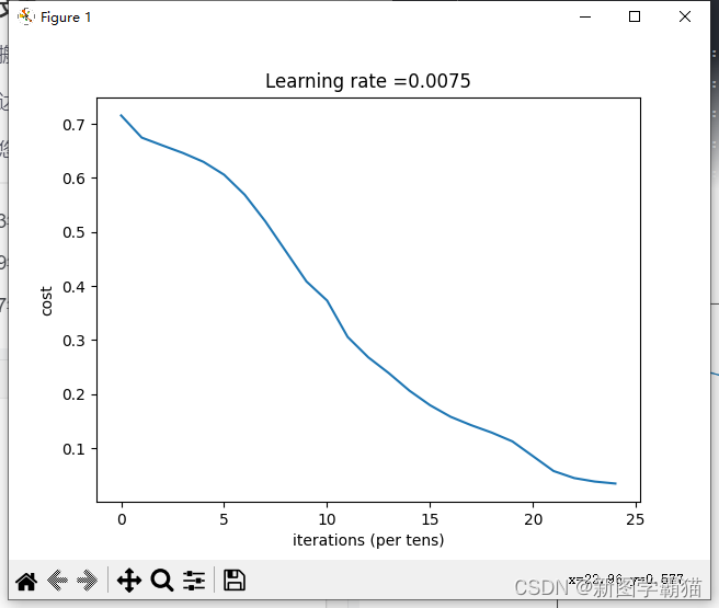
def L_layer_model(X, Y, layers_dims, learning_rate=0.0075, num_iterations=3000, print_cost=False, isPlot=True):

    np.random.seed(1)
    costs = []

    parameters = initialize_parameters_deep(layers_dims)

    for i in range(0, num_iterations):
        AL, caches = L_model_forward(X, parameters)

        cost = compute_cost(AL, Y)

        grads = L_model_backward(AL, Y, caches)

        parameters = update_parameters(parameters, grads, learning_rate)

        # 打印成本值，如果print_cost=False则忽略
        if i % 100 == 0:
            # 记录成本
            costs.append(cost)
            # 是否打印成本值
            if print_cost:
                print("第", i, "次迭代，成本值为：", np.squeeze(cost))
    # 迭代完成，根据条件绘制图
    if isPlot:
        plt.plot(np.squeeze(costs))
        plt.ylabel('cost')
        plt.xlabel('iterations (per tens)')
        plt.title("Learning rate =" + str(learning_rate))
        plt.show()
    return parameters

train_set_x_orig , train_set_y , test_set_x_orig , test_set_y , classes = lr_utils.load_dataset()

train_x_flatten = train_set_x_orig.reshape(train_set_x_orig.shape[0], -1).T
test_x_flatten = test_set_x_orig.reshape(test_set_x_orig.shape[0], -1).T

train_x = train_x_flatten / 255
train_y = train_set_y
test_x = test_x_flatten / 255
test_y = test_set_y

layers_dims = [12288, 20, 7, 5, 1] #  5-layer model
parameters = L_layer_model(train_x, train_y, layers_dims, num_iterations = 2500, print_cost = True,isPlot=True)

pred_train = predict(train_x, train_y, parameters) #训练集
pred_test = predict(test_x, test_y, parameters) #测试集

testCase.py

import numpy as np


def linear_forward_test_case():
    np.random.seed(1)
    A = np.random.randn(3, 2)
    W = np.random.randn(1, 3)
    b = np.random.randn(1, 1)

    return A, W, b


def linear_activation_forward_test_case():
    np.random.seed(2)
    A_prev = np.random.randn(3, 2)
    W = np.random.randn(1, 3)
    b = np.random.randn(1, 1)
    return A_prev, W, b


def L_model_forward_test_case():
    np.random.seed(1)
    X = np.random.randn(4, 2)
    W1 = np.random.randn(3, 4)
    b1 = np.random.randn(3, 1)
    W2 = np.random.randn(1, 3)
    b2 = np.random.randn(1, 1)
    parameters = {"W1": W1,
                  "b1": b1,
                  "W2": W2,
                  "b2": b2}

    return X, parameters


def compute_cost_test_case():
    Y = np.asarray([[1, 1, 1]])
    aL = np.array([[.8, .9, 0.4]])

    return Y, aL


def linear_backward_test_case():
    np.random.seed(1)
    dZ = np.random.randn(1, 2)
    A = np.random.randn(3, 2)
    W = np.random.randn(1, 3)
    b = np.random.randn(1, 1)
    linear_cache = (A, W, b)
    return dZ, linear_cache


def linear_activation_backward_test_case():
    np.random.seed(2)
    dA = np.random.randn(1, 2)
    A = np.random.randn(3, 2)
    W = np.random.randn(1, 3)
    b = np.random.randn(1, 1)
    Z = np.random.randn(1, 2)
    linear_cache = (A, W, b)
    activation_cache = Z
    linear_activation_cache = (linear_cache, activation_cache)

    return dA, linear_activation_cache


def L_model_backward_test_case():
    np.random.seed(3)
    AL = np.random.randn(1, 2)
    Y = np.array([[1, 0]])

    A1 = np.random.randn(4, 2)
    W1 = np.random.randn(3, 4)
    b1 = np.random.randn(3, 1)
    Z1 = np.random.randn(3, 2)
    linear_cache_activation_1 = ((A1, W1, b1), Z1)

    A2 = np.random.randn(3, 2)
    W2 = np.random.randn(1, 3)
    b2 = np.random.randn(1, 1)
    Z2 = np.random.randn(1, 2)
    linear_cache_activation_2 = ((A2, W2, b2), Z2)

    caches = (linear_cache_activation_1, linear_cache_activation_2)

    return AL, Y, caches


def update_parameters_test_case():
    np.random.seed(2)
    W1 = np.random.randn(3, 4)
    b1 = np.random.randn(3, 1)
    W2 = np.random.randn(1, 3)
    b2 = np.random.randn(1, 1)
    parameters = {"W1": W1,
                  "b1": b1,
                  "W2": W2,
                  "b2": b2}
    np.random.seed(3)
    dW1 = np.random.randn(3, 4)
    db1 = np.random.randn(3, 1)
    dW2 = np.random.randn(1, 3)
    db2 = np.random.randn(1, 1)
    grads = {"dW1": dW1,
             "db1": db1,
             "dW2": dW2,
             "db2": db2}

    return parameters, grads

dnn_utils.py

# dnn_utils.py
import numpy as np

def sigmoid(Z):
    """
    Implements the sigmoid activation in numpy

    Arguments:
    Z -- numpy array of any shape

    Returns:
    A -- output of sigmoid(z), same shape as Z
    cache -- returns Z as well, useful during backpropagation
    """

    A = 1/(1+np.exp(-Z))
    cache = Z

    return A, cache

def sigmoid_backward(dA, cache):
    """
    Implement the backward propagation for a single SIGMOID unit.

    Arguments:
    dA -- post-activation gradient, of any shape
    cache -- 'Z' where we store for computing backward propagation efficiently

    Returns:
    dZ -- Gradient of the cost with respect to Z
    """

    Z = cache

    s = 1/(1+np.exp(-Z))
    dZ = dA * s * (1-s)

    assert (dZ.shape == Z.shape)

    return dZ

def relu(Z):
    """
    Implement the RELU function.

    Arguments:
    Z -- Output of the linear layer, of any shape

    Returns:
    A -- Post-activation parameter, of the same shape as Z
    cache -- a python dictionary containing "A" ; stored for computing the backward pass efficiently
    """

    A = np.maximum(0,Z)

    assert(A.shape == Z.shape)

    cache = Z
    return A, cache

def relu_backward(dA, cache):
    """
    Implement the backward propagation for a single RELU unit.

    Arguments:
    dA -- post-activation gradient, of any shape
    cache -- 'Z' where we store for computing backward propagation efficiently

    Returns:
    dZ -- Gradient of the cost with respect to Z
    """

    Z = cache
    dZ = np.array(dA, copy=True) # just converting dz to a correct object.

    # When z <= 0, you should set dz to 0 as well.
    dZ[Z <= 0] = 0

    assert (dZ.shape == Z.shape)

    return dZ

lr_utils.py

import numpy as np
import h5py


def load_dataset():
    train_dataset = h5py.File('datasets/train_catvnoncat.h5', "r")
    train_set_x_orig = np.array(train_dataset["train_set_x"][:])  # your train set features
    train_set_y_orig = np.array(train_dataset["train_set_y"][:])  # your train set labels

    test_dataset = h5py.File('datasets/test_catvnoncat.h5', "r")
    test_set_x_orig = np.array(test_dataset["test_set_x"][:])  # your test set features
    test_set_y_orig = np.array(test_dataset["test_set_y"][:])  # your test set labels

    classes = np.array(test_dataset["list_classes"][:])  # the list of classes

    train_set_y_orig = train_set_y_orig.reshape((1, train_set_y_orig.shape[0]))
    test_set_y_orig = test_set_y_orig.reshape((1, test_set_y_orig.shape[0]))

    return train_set_x_orig, train_set_y_orig, test_set_x_orig, test_set_y_orig, classes

在这里插入图片描述

吴恩达深度学习课程二第一周作业

import numpy as np
import matplotlib.pyplot as plt
import sklearn
import sklearn.datasets
import init_utils   #第一部分，初始化
import reg_utils    #第二部分，正则化
import gc_utils     #第三部分，梯度校验
#%matplotlib inline #如果你使用的是Jupyter Notebook，请取消注释。
plt.rcParams['figure.figsize'] = (7.0, 4.0) # set default size of plots
plt.rcParams['image.interpolation'] = 'nearest'
plt.rcParams['image.cmap'] = 'gray'

train_X, train_Y, test_X, test_Y = init_utils.load_dataset(is_plot=True)


def model(X, Y, learning_rate=0.01, num_iterations=15000, print_cost=True, initialization="he", is_polt=True):
    """
    实现一个三层的神经网络：LINEAR ->RELU -> LINEAR -> RELU -> LINEAR -> SIGMOID

    参数：
        X - 输入的数据，维度为(2, 要训练/测试的数量)
        Y - 标签，【0 | 1】，维度为(1，对应的是输入的数据的标签)
        learning_rate - 学习速率
        num_iterations - 迭代的次数
        print_cost - 是否打印成本值，每迭代1000次打印一次
        initialization - 字符串类型，初始化的类型【"zeros" | "random" | "he"】
        is_polt - 是否绘制梯度下降的曲线图
    返回
        parameters - 学习后的参数
    """
    grads = {}
    costs = []
    m = X.shape[1]
    layers_dims = [X.shape[0], 10, 5, 1]

    # 选择初始化参数的类型
    if initialization == "zeros":
        parameters = initialize_parameters_zeros(layers_dims)
    elif initialization == "random":
        parameters = initialize_parameters_random(layers_dims)
    elif initialization == "he":
        parameters = initialize_parameters_he(layers_dims)
    else:
        print("错误的初始化参数！程序退出")
        exit

    # 开始学习
    for i in range(0, num_iterations):
        # 前向传播
        a3, cache = init_utils.forward_propagation(X, parameters)

        # 计算成本
        cost = init_utils.compute_loss(a3, Y)

        # 反向传播
        grads = init_utils.backward_propagation(X, Y, cache)

        # 更新参数
        parameters = init_utils.update_parameters(parameters, grads, learning_rate)

        # 记录成本
        if i % 1000 == 0:
            costs.append(cost)
            # 打印成本
            if print_cost:
                print("第" + str(i) + "次迭代，成本值为：" + str(cost))

    # 学习完毕，绘制成本曲线
    if is_polt:
        plt.plot(costs)
        plt.ylabel('cost')
        plt.xlabel('iterations (per hundreds)')
        plt.title("Learning rate =" + str(learning_rate))
        plt.show()

    # 返回学习完毕后的参数
    return parameters


def initialize_parameters_zeros(layers_dims):
    """
    将模型的参数全部设置为0

    参数：
        layers_dims - 列表，模型的层数和对应每一层的节点的数量
    返回
        parameters - 包含了所有W和b的字典
            W1 - 权重矩阵，维度为（layers_dims[1], layers_dims[0]）
            b1 - 偏置向量，维度为（layers_dims[1],1）
            ···
            WL - 权重矩阵，维度为（layers_dims[L], layers_dims[L -1]）
            bL - 偏置向量，维度为（layers_dims[L],1）
    """
    parameters = {}

    L = len(layers_dims)  # 网络层数

    for l in range(1, L):
        parameters["W" + str(l)] = np.zeros((layers_dims[l], layers_dims[l - 1]))
        parameters["b" + str(l)] = np.zeros((layers_dims[l], 1))

        # 使用断言确保我的数据格式是正确的
        assert (parameters["W" + str(l)].shape == (layers_dims[l], layers_dims[l - 1]))
        assert (parameters["b" + str(l)].shape == (layers_dims[l], 1))

    return parameters

parameters = model(train_X, train_Y, initialization = "zeros",is_polt=True)

# print ("训练集:")
# predictions_train = init_utils.predict(train_X, train_Y, parameters)
# print ("测试集:")
# predictions_test = init_utils.predict(test_X, test_Y, parameters)
#
# print("predictions_train = " + str(predictions_train))
# print("predictions_test = " + str(predictions_test))
#
# plt.title("Model with Zeros initialization")
# axes = plt.gca()
# axes.set_xlim([-1.5, 1.5])
# axes.set_ylim([-1.5, 1.5])
# init_utils.plot_decision_boundary(lambda x: init_utils.predict_dec(parameters, x.T), train_X, train_Y)


def initialize_parameters_random(layers_dims):
    """
    参数：
        layers_dims - 列表，模型的层数和对应每一层的节点的数量
    返回
        parameters - 包含了所有W和b的字典
            W1 - 权重矩阵，维度为（layers_dims[1], layers_dims[0]）
            b1 - 偏置向量，维度为（layers_dims[1],1）
            ···
            WL - 权重矩阵，维度为（layers_dims[L], layers_dims[L -1]）
            b1 - 偏置向量，维度为（layers_dims[L],1）
    """

    np.random.seed(3)  # 指定随机种子
    parameters = {}
    L = len(layers_dims)  # 层数

    for l in range(1, L):
        parameters['W' + str(l)] = np.random.randn(layers_dims[l], layers_dims[l - 1]) * 10  # 使用10倍缩放
        parameters['b' + str(l)] = np.zeros((layers_dims[l], 1))

        # 使用断言确保我的数据格式是正确的
        assert (parameters["W" + str(l)].shape == (layers_dims[l], layers_dims[l - 1]))
        assert (parameters["b" + str(l)].shape == (layers_dims[l], 1))

    return parameters

# parameters = initialize_parameters_random([3, 2, 1])
# print("W1 = " + str(parameters["W1"]))
# print("b1 = " + str(parameters["b1"]))
# print("W2 = " + str(parameters["W2"]))
# print("b2 = " + str(parameters["b2"]))

# parameters = model(train_X, train_Y, initialization = "random",is_polt=True)
# print("训练集：")
# predictions_train = init_utils.predict(train_X, train_Y, parameters)
# print("测试集：")
# predictions_test = init_utils.predict(test_X, test_Y, parameters)
#
# print(predictions_train)
# print(predictions_test)
#
#
# plt.title("Model with large random initialization")
# axes = plt.gca()
# axes.set_xlim([-1.5, 1.5])
# axes.set_ylim([-1.5, 1.5])
# init_utils.plot_decision_boundary(lambda x: init_utils.predict_dec(parameters, x.T), train_X, train_Y)

def initialize_parameters_he(layers_dims):
    """
    参数：
        layers_dims - 列表，模型的层数和对应每一层的节点的数量
    返回
        parameters - 包含了所有W和b的字典
            W1 - 权重矩阵，维度为（layers_dims[1], layers_dims[0]）
            b1 - 偏置向量，维度为（layers_dims[1],1）
            ···
            WL - 权重矩阵，维度为（layers_dims[L], layers_dims[L -1]）
            b1 - 偏置向量，维度为（layers_dims[L],1）
    """

    np.random.seed(3)  # 指定随机种子
    parameters = {}
    L = len(layers_dims)  # 层数

    for l in range(1, L):
        parameters['W' + str(l)] = np.random.randn(layers_dims[l], layers_dims[l - 1]) * np.sqrt(2 / layers_dims[l - 1])
        parameters['b' + str(l)] = np.zeros((layers_dims[l], 1))

        # 使用断言确保我的数据格式是正确的
        assert (parameters["W" + str(l)].shape == (layers_dims[l], layers_dims[l - 1]))
        assert (parameters["b" + str(l)].shape == (layers_dims[l], 1))

    return parameters

# parameters = initialize_parameters_he([2, 4, 1])
# print("W1 = " + str(parameters["W1"]))
# print("b1 = " + str(parameters["b1"]))
# print("W2 = " + str(parameters["W2"]))
# print("b2 = " + str(parameters["b2"]))
#
# parameters = model(train_X, train_Y, initialization = "he",is_polt=True)
# print("训练集:")
# predictions_train = init_utils.predict(train_X, train_Y, parameters)
# print("测试集:")
# init_utils.predictions_test = init_utils.predict(test_X, test_Y, parameters)
#
# plt.title("Model with He initialization")
# axes = plt.gca()
# axes.set_xlim([-1.5, 1.5])
# axes.set_ylim([-1.5, 1.5])
# init_utils.plot_decision_boundary(lambda x: init_utils.predict_dec(parameters, x.T), train_X, train_Y)

课程二第二周作业

# -*- coding: utf-8 -*-

import numpy as np
import matplotlib.pyplot as plt
import scipy.io
import math
import sklearn
import sklearn.datasets

import opt_utils #参见数据包或者在本文底部copy
import testCase  #参见数据包或者在本文底部copy

#%matplotlib inline #如果你用的是Jupyter Notebook请取消注释
plt.rcParams['figure.figsize'] = (7.0, 4.0) # set default size of plots
plt.rcParams['image.interpolation'] = 'nearest'
plt.rcParams['image.cmap'] = 'gray'


#梯度下降
def update_parameters_with_gd(parameters, grads, learning_rate):

    L = len(parameters) // 2  # 神经网络的层数

    # 更新每个参数
    for l in range(L):
        parameters["W" + str(l + 1)] = parameters["W" + str(l + 1)] - learning_rate * grads["dW" + str(l + 1)]
        parameters["b" + str(l + 1)] = parameters["b" + str(l + 1)] - learning_rate * grads["db" + str(l + 1)]

    return parameters


# #测试update_parameters_with_gd
# print("-------------测试update_parameters_with_gd-------------")
# parameters , grads , learning_rate = testCase.update_parameters_with_gd_test_case()
# parameters = update_parameters_with_gd(parameters,grads,learning_rate)
# print("W1 = " + str(parameters["W1"]))
# print("b1 = " + str(parameters["b1"]))
# print("W2 = " + str(parameters["W2"]))
# print("b2 = " + str(parameters["b2"]))


def random_mini_batches(X, Y, mini_batch_size=64, seed=0):

    np.random.seed(seed)  # 指定随机种子
    m = X.shape[1]
    mini_batches = []

    # 第一步：打乱顺序
    permutation = list(np.random.permutation(m))  # 它会返回一个长度为m的随机数组，且里面的数是0到m-1
    shuffled_X = X[:, permutation]  # 将每一列的数据按permutation的顺序来重新排列。
    shuffled_Y = Y[:, permutation].reshape((1, m))

    # 第二步，分割
    num_complete_minibatches = math.floor(m / mini_batch_size)  # 把你的训练集分割成多少份,请注意，如果值是99.99，那么返回值是99，剩下的0.99会被舍弃
    for k in range(0, num_complete_minibatches):
        mini_batch_X = shuffled_X[:, k * mini_batch_size:(k + 1) * mini_batch_size]
        mini_batch_Y = shuffled_Y[:, k * mini_batch_size:(k + 1) * mini_batch_size]

        mini_batch = (mini_batch_X, mini_batch_Y)
        mini_batches.append(mini_batch)

    # 如果训练集的大小刚好是mini_batch_size的整数倍，那么这里已经处理完了
    # 如果训练集的大小不是mini_batch_size的整数倍，那么最后肯定会剩下一些，我们要把它处理了
    if m % mini_batch_size != 0:
        # 获取最后剩余的部分
        mini_batch_X = shuffled_X[:, mini_batch_size * num_complete_minibatches:]
        mini_batch_Y = shuffled_Y[:, mini_batch_size * num_complete_minibatches:]

        mini_batch = (mini_batch_X, mini_batch_Y)
        mini_batches.append(mini_batch)

    return mini_batches


# #测试random_mini_batches
# print("-------------测试random_mini_batches-------------")
# X_assess,Y_assess,mini_batch_size = testCase.random_mini_batches_test_case()
# mini_batches = random_mini_batches(X_assess,Y_assess,mini_batch_size)
#
# print("第1个mini_batch_X 的维度为：",mini_batches[0][0].shape)
# print("第1个mini_batch_Y 的维度为：",mini_batches[0][1].shape)
# print("第2个mini_batch_X 的维度为：",mini_batches[1][0].shape)
# print("第2个mini_batch_Y 的维度为：",mini_batches[1][1].shape)
# print("第3个mini_batch_X 的维度为：",mini_batches[2][0].shape)
# print("第3个mini_batch_Y 的维度为：",mini_batches[2][1].shape)

def initialize_velocity(parameters):

    L = len(parameters) // 2  # 神经网络的层数
    v = {}

    for l in range(L):
        v["dW" + str(l + 1)] = np.zeros_like(parameters["W" + str(l + 1)])
        v["db" + str(l + 1)] = np.zeros_like(parameters["b" + str(l + 1)])

    return v
#
# #测试initialize_velocity
# print("-------------测试initialize_velocity-------------")
# parameters = testCase.initialize_velocity_test_case()
# v = initialize_velocity(parameters)
#
# print('v["dW1"] = ' + str(v["dW1"]))
# print('v["db1"] = ' + str(v["db1"]))
# print('v["dW2"] = ' + str(v["dW2"]))
# print('v["db2"] = ' + str(v["db2"]))


def update_parameters_with_momentun(parameters, grads, v, beta, learning_rate):

    L = len(parameters) // 2
    for l in range(L):
        # 计算速度
        v["dW" + str(l + 1)] = beta * v["dW" + str(l + 1)] + (1 - beta) * grads["dW" + str(l + 1)]
        v["db" + str(l + 1)] = beta * v["db" + str(l + 1)] + (1 - beta) * grads["db" + str(l + 1)]

        # 更新参数
        parameters["W" + str(l + 1)] = parameters["W" + str(l + 1)] - learning_rate * v["dW" + str(l + 1)]
        parameters["b" + str(l + 1)] = parameters["b" + str(l + 1)] - learning_rate * v["db" + str(l + 1)]

    return parameters, v

# #测试update_parameters_with_momentun
# print("-------------测试update_parameters_with_momentun-------------")
# parameters,grads,v = testCase.update_parameters_with_momentum_test_case()
# update_parameters_with_momentun(parameters,grads,v,beta=0.9,learning_rate=0.01)
#
# print("W1 = " + str(parameters["W1"]))
# print("b1 = " + str(parameters["b1"]))
# print("W2 = " + str(parameters["W2"]))
# print("b2 = " + str(parameters["b2"]))
# print('v["dW1"] = ' + str(v["dW1"]))
# print('v["db1"] = ' + str(v["db1"]))
# print('v["dW2"] = ' + str(v["dW2"]))
# print('v["db2"] = ' + str(v["db2"]))

def initialize_adam(parameters):

    L = len(parameters) // 2
    v = {}
    s = {}

    for l in range(L):
        v["dW" + str(l + 1)] = np.zeros_like(parameters["W" + str(l + 1)])
        v["db" + str(l + 1)] = np.zeros_like(parameters["b" + str(l + 1)])

        s["dW" + str(l + 1)] = np.zeros_like(parameters["W" + str(l + 1)])
        s["db" + str(l + 1)] = np.zeros_like(parameters["b" + str(l + 1)])

    return (v, s)

# #测试initialize_adam
# print("-------------测试initialize_adam-------------")
# parameters = testCase.initialize_adam_test_case()
# v,s = initialize_adam(parameters)
#
# print('v["dW1"] = ' + str(v["dW1"]))
# print('v["db1"] = ' + str(v["db1"]))
# print('v["dW2"] = ' + str(v["dW2"]))
# print('v["db2"] = ' + str(v["db2"]))
# print('s["dW1"] = ' + str(s["dW1"]))
# print('s["db1"] = ' + str(s["db1"]))
# print('s["dW2"] = ' + str(s["dW2"]))
# print('s["db2"] = ' + str(s["db2"]))

def update_parameters_with_adam(parameters, grads, v, s, t, learning_rate=0.01, beta1=0.9, beta2=0.999, epsilon=1e-8):

    L = len(parameters) // 2
    v_corrected = {}  # 偏差修正后的值
    s_corrected = {}  # 偏差修正后的值

    for l in range(L):
        # 梯度的移动平均值,输入："v , grads , beta1",输出：" v "
        v["dW" + str(l + 1)] = beta1 * v["dW" + str(l + 1)] + (1 - beta1) * grads["dW" + str(l + 1)]
        v["db" + str(l + 1)] = beta1 * v["db" + str(l + 1)] + (1 - beta1) * grads["db" + str(l + 1)]

        # 计算第一阶段的偏差修正后的估计值，输入"v , beta1 , t" , 输出："v_corrected"
        v_corrected["dW" + str(l + 1)] = v["dW" + str(l + 1)] / (1 - np.power(beta1, t))
        v_corrected["db" + str(l + 1)] = v["db" + str(l + 1)] / (1 - np.power(beta1, t))

        # 计算平方梯度的移动平均值，输入："s, grads , beta2"，输出："s"
        s["dW" + str(l + 1)] = beta2 * s["dW" + str(l + 1)] + (1 - beta2) * np.square(grads["dW" + str(l + 1)])
        s["db" + str(l + 1)] = beta2 * s["db" + str(l + 1)] + (1 - beta2) * np.square(grads["db" + str(l + 1)])

        # 计算第二阶段的偏差修正后的估计值，输入："s , beta2 , t"，输出："s_corrected"
        s_corrected["dW" + str(l + 1)] = s["dW" + str(l + 1)] / (1 - np.power(beta2, t))
        s_corrected["db" + str(l + 1)] = s["db" + str(l + 1)] / (1 - np.power(beta2, t))

        # 更新参数，输入: "parameters, learning_rate, v_corrected, s_corrected, epsilon". 输出: "parameters".
        parameters["W" + str(l + 1)] = parameters["W" + str(l + 1)] - learning_rate * (
                    v_corrected["dW" + str(l + 1)] / np.sqrt(s_corrected["dW" + str(l + 1)] + epsilon))
        parameters["b" + str(l + 1)] = parameters["b" + str(l + 1)] - learning_rate * (
                    v_corrected["db" + str(l + 1)] / np.sqrt(s_corrected["db" + str(l + 1)] + epsilon))

    return (parameters, v, s)

# #测试update_with_parameters_with_adam
# print("-------------测试update_with_parameters_with_adam-------------")
# parameters , grads , v , s = testCase.update_parameters_with_adam_test_case()
# update_parameters_with_adam(parameters,grads,v,s,t=2)
#
# print("W1 = " + str(parameters["W1"]))
# print("b1 = " + str(parameters["b1"]))
# print("W2 = " + str(parameters["W2"]))
# print("b2 = " + str(parameters["b2"]))
# print('v["dW1"] = ' + str(v["dW1"]))
# print('v["db1"] = ' + str(v["db1"]))
# print('v["dW2"] = ' + str(v["dW2"]))
# print('v["db2"] = ' + str(v["db2"]))
# print('s["dW1"] = ' + str(s["dW1"]))
# print('s["db1"] = ' + str(s["db1"]))
# print('s["dW2"] = ' + str(s["dW2"]))
# print('s["db2"] = ' + str(s["db2"]))

train_X, train_Y = opt_utils.load_dataset(is_plot=True)


def model(X, Y, layers_dims, optimizer, learning_rate=0.0007,
          mini_batch_size=64, beta=0.9, beta1=0.9, beta2=0.999,
          epsilon=1e-8, num_epochs=10000, print_cost=True, is_plot=True):

    L = len(layers_dims)
    costs = []
    t = 0  # 每学习完一个minibatch就增加1
    seed = 10  # 随机种子

    # 初始化参数
    parameters = opt_utils.initialize_parameters(layers_dims)

    # 选择优化器
    if optimizer == "gd":
        pass  # 不使用任何优化器，直接使用梯度下降法
    elif optimizer == "momentum":
        v = initialize_velocity(parameters)  # 使用动量
    elif optimizer == "adam":
        v, s = initialize_adam(parameters)  # 使用Adam优化
    else:
        print("optimizer参数错误，程序退出。")
        exit(1)

    # 开始学习
    for i in range(num_epochs):
        # 定义随机 minibatches,我们在每次遍历数据集之后增加种子以重新排列数据集，使每次数据的顺序都不同
        seed = seed + 1
        minibatches = random_mini_batches(X, Y, mini_batch_size, seed)

        for minibatch in minibatches:
            # 选择一个minibatch
            (minibatch_X, minibatch_Y) = minibatch

            # 前向传播
            A3, cache = opt_utils.forward_propagation(minibatch_X, parameters)

            # 计算误差
            cost = opt_utils.compute_cost(A3, minibatch_Y)

            # 反向传播
            grads = opt_utils.backward_propagation(minibatch_X, minibatch_Y, cache)

            # 更新参数
            if optimizer == "gd":
                parameters = update_parameters_with_gd(parameters, grads, learning_rate)
            elif optimizer == "momentum":
                parameters, v = update_parameters_with_momentun(parameters, grads, v, beta, learning_rate)
            elif optimizer == "adam":
                t = t + 1
                parameters, v, s = update_parameters_with_adam(parameters, grads, v, s, t, learning_rate, beta1, beta2,
                                                               epsilon)
        # 记录误差值
        if i % 100 == 0:
            costs.append(cost)
            # 是否打印误差值
            if print_cost and i % 1000 == 0:
                print("第" + str(i) + "次遍历整个数据集，当前误差值：" + str(cost))
    # 是否绘制曲线图
    if is_plot:
        plt.plot(costs)
        plt.ylabel('cost')
        plt.xlabel('epochs (per 100)')
        plt.title("Learning rate = " + str(learning_rate))
        plt.show()

    return parameters





#使用普通的梯度下降
layers_dims = [train_X.shape[0],5,2,1]
parameters = model(train_X, train_Y, layers_dims, optimizer="gd",is_plot=True)
#预测
preditions = opt_utils.predict(train_X,train_Y,parameters)
#绘制分类图
plt.title("Model with Gradient Descent optimization")
axes = plt.gca()
axes.set_xlim([-1.5, 2.5])
axes.set_ylim([-1, 1.5])
opt_utils.plot_decision_boundary(lambda x: opt_utils.predict_dec(parameters, x.T), train_X, train_Y)





layers_dims = [train_X.shape[0],5,2,1]
#使用动量的梯度下降
parameters = model(train_X, train_Y, layers_dims, beta=0.9,optimizer="momentum",is_plot=True)
#预测
preditions = opt_utils.predict(train_X,train_Y,parameters)
#绘制分类图
plt.title("Model with Momentum optimization")
axes = plt.gca()
axes.set_xlim([-1.5, 2.5])
axes.set_ylim([-1, 1.5])
opt_utils.plot_decision_boundary(lambda x: opt_utils.predict_dec(parameters, x.T), train_X, train_Y)





layers_dims = [train_X.shape[0], 5, 2, 1]
#使用Adam优化的梯度下降
parameters = model(train_X, train_Y, layers_dims, optimizer="adam",is_plot=True)
#预测
preditions = opt_utils.predict(train_X,train_Y,parameters)
#绘制分类图
plt.title("Model with Adam optimization")
axes = plt.gca()
axes.set_xlim([-1.5, 2.5])
axes.set_ylim([-1, 1.5])
opt_utils.plot_decision_boundary(lambda x: opt_utils.predict_dec(parameters, x.T), train_X, train_Y)

课程二第三周作业

import math

import matplotlib
import numpy as np
import h5py
import matplotlib.pyplot as plt
import tensorflow as tf
from tensorflow.python.framework import ops
import tf_utils
import time

%matplotlib inline
np.random.seed(1)

a = tf.constant(2)
b = tf.constant(10)
c = tf.multiply(a,b)

print(c)

sess = tf.Session()

print(sess.run(c))

#利用feed_dict来改变x的值
x = tf.placeholder(tf.int64,name="x")
print(sess.run(2 * x,feed_dict={x:3}))
sess.close()


def linear_function():

    np.random.seed(1)  # 指定随机种子

    X = np.random.randn(3, 1)
    W = np.random.randn(4, 3)
    b = np.random.randn(4, 1)

    Y = tf.add(tf.matmul(W, X), b)  # tf.matmul是矩阵乘法
    # Y = tf.matmul(W,X) + b #也可以以写成这样子

    # 创建一个session并运行它
    sess = tf.Session()
    result = sess.run(Y)

    # session使用完毕，关闭它
    sess.close()

    return result

print("=====我们来测试一下=====")
print("result = " +  str(linear_function()))


def sigmoid(z):
    """
    实现使用sigmoid函数计算z

    参数：
        z - 输入的值，标量或矢量

    返回：
        result - 用sigmoid计算z的值

    """

    # 创建一个占位符x，名字叫“x”
    x = tf.placeholder(tf.float32, name="x")

    # 计算sigmoid(z)
    sigmoid = tf.sigmoid(x)

    # 创建一个会话，使用方法二
    with tf.Session() as sess:
        result = sess.run(sigmoid, feed_dict={x: z})

    return result

print("=====我们来测试一下=====")
print ("sigmoid(0) = " + str(sigmoid(0)))
print ("sigmoid(12) = " + str(sigmoid(12)))


def one_hot_matrix(lables, C):
    """
    创建一个矩阵，其中第i行对应第i个类号，第j列对应第j个训练样本
    所以如果第j个样本对应着第i个标签，那么entry (i,j)将会是1

    参数：
        lables - 标签向量
        C - 分类数

    返回：
        one_hot - 独热矩阵

    """

    # 创建一个tf.constant，赋值为C，名字叫C
    C = tf.constant(C, name="C")

    # 使用tf.one_hot，注意一下axis
    one_hot_matrix = tf.one_hot(indices=lables, depth=C, axis=0)

    # 创建一个session
    sess = tf.Session()

    # 运行session
    one_hot = sess.run(one_hot_matrix)

    # 关闭session
    sess.close()

    return one_hot

print("=====我们测试一下=====")
labels = np.array([1,2,3,0,2,1])
one_hot = one_hot_matrix(labels,C=4)
print(str(one_hot))


def ones(shape):
    """
    创建一个维度为shape的变量，其值全为1

    参数：
        shape - 你要创建的数组的维度

    返回：
        ones - 只包含1的数组
    """

    # 使用tf.ones()
    ones = tf.ones(shape)

    # 创建会话
    sess = tf.Session()

    # 运行会话
    ones = sess.run(ones)

    # 关闭会话
    sess.close()

    return ones

print ("ones = " + str(ones([3])))

# 定义 y_hat 为固定值 36
y_hat = tf.constant(36, name = "y_hat")
# 定义 y 为固定值 39
y = tf.constant(39,name = "y")

# 为损失函数创建一个变量
loss = tf.Variable((y-y_hat)**2,name = "loss" )
# 运行之后的初始化(ession.run(init))
# 损失变量将被初始化并准备计算
init = tf.global_variables_initializer()

# 创建一个 session 并打印输出
with tf.Session() as session:
    ## 初始化变量
    session.run(init)
    ## 打印损失值
    print(session.run(loss))


def cost(logits, labels):

    ### START CODE HERE ###

    # Create the placeholders for "logits" (z) and "labels" (y) (approx. 2 lines)
    z = tf.placeholder(tf.float32, name="z")
    y = tf.placeholder(tf.float32, name="y")

    # Use the loss function (approx. 1 line)
    cost = tf.nn.sigmoid_cross_entropy_with_logits(logits=z, labels=y)

    # Create a session (approx. 1 line). See method 1 above.
    sess = tf.Session()

    # Run the session (approx. 1 line).
    cost = sess.run(cost, feed_dict={z: logits, y: labels})

    # Close the session (approx. 1 line). See method 1 above.
    sess.close()

    ### END CODE HERE ###

    return cost

X_train_orig , Y_train_orig , X_test_orig , Y_test_orig , classes = tf_utils.load_dataset()
#查看数据集
index = 11
plt.imshow(X_train_orig[index])
print("Y = " + str(np.squeeze(Y_train_orig[:,index])))
#数据集扁平化
# 每一列就是一个样本
X_train_flatten = X_train_orig.reshape(X_train_orig.shape[0],-1).T
X_test_flatten = X_test_orig.reshape(X_test_orig.shape[0],-1).T

# 归一化数据
X_train = X_train_flatten / 255
X_test = X_test_flatten / 255

# 转换为独热矩阵
Y_train = tf_utils.convert_to_one_hot(Y_train_orig,6)
Y_test = tf_utils.convert_to_one_hot(Y_test_orig,6)

print("训练集样本数 = " + str(X_train.shape[1]))
print("测试集样本数 = " + str(X_test.shape[1]))
print("X_train.shape: " + str(X_train.shape))
print("Y_train.shape: " + str(Y_train.shape))
print("X_test.shape: " + str(X_test.shape))
print("Y_test.shape: " + str(Y_test.shape))

#创建占位符
def create_placeholders(n_x, n_y):
    X = tf.placeholder(tf.float32, [n_x, None], name="X")
    Y = tf.placeholder(tf.float32, [n_y, None], name="Y")

    return X, Y
print("=====我们测试一下=====")
X, Y = create_placeholders(12288, 6)
print ("X = " + str(X))
print ("Y = " + str(Y))

#初始化参数
W1 = tf.get_variable("W1", [25,12288], initializer = tf.contrib.layers.xavier_initializer(seed = 1))
b1 = tf.get_variable("b1", [25,1], initializer = tf.zeros_initializer())


def initialize_parameters():
    tf.set_random_seed(1)  # 指定随机种子

    W1 = tf.get_variable("W1", [25, 12288], initializer=tf.contrib.layers.xavier_initializer(seed=1))
    b1 = tf.get_variable("b1", [25, 1], initializer=tf.zeros_initializer())
    W2 = tf.get_variable("W2", [12, 25], initializer=tf.contrib.layers.xavier_initializer(seed=1))
    b2 = tf.get_variable("b2", [12, 1], initializer=tf.zeros_initializer())
    W3 = tf.get_variable("W3", [6, 12], initializer=tf.contrib.layers.xavier_initializer(seed=1))
    b3 = tf.get_variable("b3", [6, 1], initializer=tf.zeros_initializer())

    parameters = {"W1": W1,
                  "b1": b1,
                  "W2": W2,
                  "b2": b2,
                  "W3": W3,
                  "b3": b3}

    return parameters

print("=====我们测试一下=====")
tf.reset_default_graph() #用于清除默认图形堆栈并重置全局默认图形。
with tf.Session() as sess:
    parameters = initialize_parameters()
    print("W1 = " + str(parameters["W1"]))
    print("b1 = " + str(parameters["b1"]))
    print("W2 = " + str(parameters["W2"]))
    print("b2 = " + str(parameters["b2"]))

#正向传播
def forward_propagation(X, parameters):
    W1 = parameters['W1']
    b1 = parameters['b1']
    W2 = parameters['W2']
    b2 = parameters['b2']
    W3 = parameters['W3']
    b3 = parameters['b3']

    Z1 = tf.add(tf.matmul(W1, X), b1)  # Z1 = np.dot(W1, X) + b1
    # Z1 = tf.matmul(W1,X) + b1             #也可以这样写
    A1 = tf.nn.relu(Z1)  # A1 = relu(Z1)
    Z2 = tf.add(tf.matmul(W2, A1), b2)  # Z2 = np.dot(W2, a1) + b2
    A2 = tf.nn.relu(Z2)  # A2 = relu(Z2)
    Z3 = tf.add(tf.matmul(W3, A2), b3)  # Z3 = np.dot(W3,Z2) + b3

    return Z3

print("=====我们测试一下=====")
tf.reset_default_graph() #用于清除默认图形堆栈并重置全局默认图形。
with tf.Session() as sess:
    X,Y = create_placeholders(12288,6)
    parameters = initialize_parameters()
    Z3 = forward_propagation(X,parameters)
    print("Z3 = " + str(Z3))

#计算损失
def compute_cost(Z3, Y):
    logits = tf.transpose(Z3)  # 转置
    labels = tf.transpose(Y)  # 转置

    cost = tf.reduce_mean(tf.nn.softmax_cross_entropy_with_logits(logits=logits, labels=labels))

    return cost

print("=====我们测试一下=====")
tf.reset_default_graph()

with tf.Session() as sess:
    X,Y = create_placeholders(12288,6)
    parameters = initialize_parameters()
    Z3 = forward_propagation(X,parameters)
    cost = compute_cost(Z3,Y)
    print("cost = " + str(cost))


def model(X_train, Y_train, X_test, Y_test,
          learning_rate=0.0001, num_epochs=1500, minibatch_size=32,
          print_cost=True, is_plot=True):

    ops.reset_default_graph()  # 能够重新运行模型而不覆盖tf变量
    tf.set_random_seed(1)
    seed = 3
    (n_x, m) = X_train.shape  # 获取输入节点数量和样本数
    n_y = Y_train.shape[0]  # 获取输出节点数量
    costs = []  # 成本集

    # 给X和Y创建placeholder
    X, Y = create_placeholders(n_x, n_y)

    # 初始化参数
    parameters = initialize_parameters()

    # 前向传播
    Z3 = forward_propagation(X, parameters)

    # 计算成本
    cost = compute_cost(Z3, Y)

    # 反向传播，使用Adam优化
    optimizer = tf.train.AdamOptimizer(learning_rate=learning_rate).minimize(cost)

    # 初始化所有的变量
    init = tf.global_variables_initializer()

    # 开始会话并计算
    with tf.Session() as sess:
        # 初始化
        sess.run(init)

        # 正常训练的循环
        for epoch in range(num_epochs):

            epoch_cost = 0  # 每代的成本
            num_minibatches = int(m / minibatch_size)  # minibatch的总数量
            seed = seed + 1
            minibatches = tf_utils.random_mini_batches(X_train, Y_train, minibatch_size, seed)

            for minibatch in minibatches:
                # 选择一个minibatch
                (minibatch_X, minibatch_Y) = minibatch

                # 数据已经准备好了，开始运行session
                _, minibatch_cost = sess.run([optimizer, cost], feed_dict={X: minibatch_X, Y: minibatch_Y})

                # 计算这个minibatch在这一代中所占的误差
                epoch_cost = epoch_cost + minibatch_cost / num_minibatches

            # 记录并打印成本
            ## 记录成本
            if epoch % 5 == 0:
                costs.append(epoch_cost)
                # 是否打印：
                if print_cost and epoch % 100 == 0:
                    print("epoch = " + str(epoch) + "    epoch_cost = " + str(epoch_cost))

        # 是否绘制图谱
        if is_plot:
            plt.plot(np.squeeze(costs))
            plt.ylabel('cost')
            plt.xlabel('iterations (per tens)')
            plt.title("Learning rate =" + str(learning_rate))
            plt.show()

        # 保存学习后的参数
        parameters = sess.run(parameters)
        print("参数已经保存到session。")

        # 计算当前的预测结果
        correct_prediction = tf.equal(tf.argmax(Z3), tf.argmax(Y))

        # 计算准确率
        accuracy = tf.reduce_mean(tf.cast(correct_prediction, "float"))

        print("训练集的准确率：", accuracy.eval({X: X_train, Y: Y_train}))
        print("测试集的准确率:", accuracy.eval({X: X_test, Y: Y_test}))

        return parameters

print("=====我们测试一下=====")
# 开始时间
start_time = time.perf_counter()
# 开始训练
parameters = model(X_train, Y_train, X_test, Y_test)
# 结束时间
end_time = time.perf_counter()
# 计算时差
print("CPU的执行时间 = " + str(end_time - start_time) + " 秒" )