数据分析第四次实训

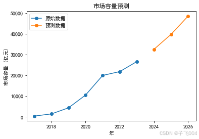
第一题

import matplotlib.pyplot as plt

# 原始数据
years = [2017, 2018, 2019, 2020, 2021, 2022, 2023]
market_capacity = [366.0, 1400.0, 4338.0, 10500.0, 19950.0, 21791.2, 26618]

# 预测依据：假设市场容量每年按照固定的增长率增长
growth_rate = (market_capacity[-1] / market_capacity[-2]) ** (1 / (years[-1] - years[-2])) - 1

# 预测未来几年的数据
predicted_years = [2024, 2025, 2026]
predicted_market_capacity = [market_capacity[-1] * (1 + growth_rate) ** (year - years[-1]) for year in predicted_years]

# 绘制原始数据和预测数据的折线图
plt.plot(years, market_capacity, marker='o', label='原始数据')
plt.plot(predicted_years, predicted_market_capacity, marker='o', label='预测数据')
plt.xlabel('年')
plt.ylabel('市场容量 (亿元)')
plt.title('市场容量预测')
plt.rcParams['font.sans-serif']=['SimHei']
plt.legend()
plt.show()

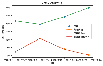
第二题

import matplotlib.pyplot as plt

# 日期数据
dates = ['2022/3/1 - 2022/3/7', '2022/3/8 - 2022/3/14', '2022/3/15 - 2022/3/21', '2022/3/22 - 2022/3/28']

# 竞店支付转化指数数据
competitor_index = [916, 895, 941, 998]

# 自身店铺支付转化指数数据
own_index = [722, 806, 738, 702]

# 绘制折线图
plt.plot(dates, competitor_index, marker='o', label='竞店')
plt.plot(dates, own_index, marker='o', label='自身店铺')

# 绘制线性图（假设线性图就是折线图）
plt.plot(dates, competitor_index, linestyle='-', label='竞店线性图')
plt.plot(dates, own_index, linestyle='-', label='自身店铺线性图')

# 添加图例
plt.legend()

# 添加标题和坐标轴标签
plt.title('支付转化指数分析')
plt.xlabel('日期')
plt.ylabel('支付转化指数')

# 显示图形
plt.show()

第三题

import pandas as pd
import matplotlib.pyplot as plt

# 读取数据
data = pd.read_excel(r'C:\Users\XXGC\Desktop\任务3竞品数据分析-素材3.xlsm')  
df = pd.DataFrame(data)

# 分析销售渠道
sales_channel_counts = df['流量渠道2'].value_counts()
print("销售渠道分析：")
print(sales_channel_counts)

# 分析流量渠道
traffic_channel_counts = df[['流量渠道3', '流量渠道4', '流量渠道5']].apply(pd.Series.value_counts).sum(axis=1)
print("\n流量渠道分析：")
print(traffic_channel_counts)

# 分析成交词
top_words = df[['成交词1', '成交词2', '成交词3']].stack().value_counts().head(10)
print("\n成交词分析：")
print(top_words)

# 作图
plt.figure(figsize=(10, 6))
sales_channel_counts.plot(kind='bar', color='skyblue')
plt.title('销售渠道分布')
plt.xlabel('销售渠道')
plt.ylabel('数量')
plt.show()

plt.figure(figsize=(10, 6))
traffic_channel_counts.plot(kind='bar', color='lightgreen')
plt.title('流量渠道分布')
plt.xlabel('流量渠道')
plt.ylabel('数量')
plt.show()

plt.figure(figsize=(10, 6))
top_words.plot(kind='bar')
plt.title('成交词分析')
plt.xlabel('成交词')
plt.ylabel('出现次数')
plt.xticks(rotation=45)
plt.show()

# 得出自身店铺优化策略
optimization_strategies = [
    "1. 优化产品价格，根据竞品价格调整自身店铺产品的定价策略，以提高竞争力。",
    "2. 加大对热门销售渠道（如搜索、购物车）的投入和优化，提高店铺在这些渠道的曝光率。",
    "3. 拓展流量渠道，尝试开发其他潜在的流量来源，如淘宝客、手淘首页等。",
    "4. 针对热门成交词，优化产品标题和描述，提高产品在搜索结果中的相关性。",
    "5. 提升产品质量和服务，以提高用户满意度和口碑，促进销量增长。",
    "6. 分析竞品的优势和不足，借鉴其成功经验，改进自身店铺的产品和运营策略。"
]

print("\n自身店铺优化策略：")
for strategy in optimization_strategies:
    print(strategy)

第四题

import pandas as pd
import matplotlib.pyplot as plt

# 读取数据
data = {
    '商品': ['白色衬衣', '黑色衬衣', '红色衬衣', '黄色衬衣', '蓝色衬衣', '绿色衬衣'],
    '访客数 /人': [1809, 2083, 679, 1918, 492, 261],
    '支付金额 /元': [27356, 27812, 6985, 30126, 5821, 3192],
    '支付件数 /件': [447, 424, 98, 443, 89, 47],
    '支付买家数 /件': [212, 231, 78, 197, 58, 32],
    '加购件数 /件': [583, 521, 294, 567, 214, 85],
    '加购人数 /人': [308, 456, 175, 435, 99, 55],
    '收藏人数 /人': [421, 376, 152, 379, 105, 86]
}
df = pd.DataFrame(data)

# 计算支付转化率
df['支付转化率'] = df['支付买家数 /件'] / df['访客数 /人']

# 计算加购转化率
df['加购转化率'] = df['加购人数 /人'] / df['访客数 /人']

# 计算收藏转化率
df['收藏转化率'] = df['收藏人数 /人'] / df['访客数 /人']

# 绘制支付金额图
plt.figure(figsize=(8, 6))
plt.bar(df['商品'], df['支付金额 /元'], color='blue')
plt.xlabel('商品')
plt.ylabel('支付金额（元）')
plt.title('支付金额分析')
plt.show() 

# 绘制收藏转化率图
plt.figure(figsize=(8, 6))
plt.plot(df['商品'], df['收藏转化率'], marker='o', color='green')
plt.xlabel('商品')
plt.ylabel('收藏转化率')
plt.title('收藏转化率分析')
plt.show()  

# 绘制加购转化率图
plt.figure(figsize=(8, 6))
plt.plot(df['商品'], df['加购转化率'], marker='o', color='red')
plt.xlabel('商品')
plt.ylabel('加购转化率')
plt.title('加购转化率分析')
plt.show()  
# 绘制支付转化率图
plt.figure(figsize=(8, 6))
plt.plot(df['商品'], df['支付转化率'], marker='o', color='purple')
plt.xlabel('商品')
plt.ylabel('支付转化率')
plt.title('支付转化率分析')
plt.show()  

第五题

import pandas as pd

# 读取数据
data = pd.read_excel(r'C:\Users\XXGC\Desktop\任务5 客户忠诚度分析-素材.xlsm')
df = pd.DataFrame(data)

# 计算购买频次
purchase_frequency = df['用户名'].value_counts()

# 购买频次排名
purchase_frequency_rank = purchase_frequency.rank(ascending=False)

# 客户及购买频次
customer_purchase_frequency = purchase_frequency.reset_index()
customer_purchase_frequency.columns = ['用户名', '购买频次']

# 客户重复购买率
repeat_purchase_rate = (customer_purchase_frequency['购买频次'] > 1).mean()

# 打印分析结果
print("购买频次排名：")
print(purchase_frequency_rank)

print("\n客户及购买频次：")
print(customer_purchase_frequency)

print("\n客户重复购买率：", repeat_purchase_rate)

第六题

import pandas as pd
import datetime

# 读取数据
data = pd.read_excel(r'C:\Users\XXGC\Desktop\任务6：RFM客户细分-素材6.xlsm')
df = pd.DataFrame(data)

# 将上次交易时间转换为 datetime 格式
df['上次交易时间'] = pd.to_datetime(df['上次交易时间'])

# 计算 RFM 值
today = datetime.datetime.now()
df['R'] = (today - df['上次交易时间']).dt.days
df['F'] = df['交易笔数(F)']
df['M'] = df['交易总额(M)/元']

# 客户标签设置
def rfm_label(r, f, m):
    if r <= 30 and f >= 5 and m >= 200:
        return '重要价值客户'
    elif r <= 30 and f >= 1 and m >= 100:
        return '重要发展客户'
    elif r <= 90 and f >= 1:
        return '重要保持客户'
    elif f >= 1:
        return '重要挽留客户'
    else:
        return '一般客户'

df['客户标签'] = df.apply(lambda x: rfm_label(x['R'], x['F'], x['M']), axis=1)

# 客户评价及营销策略
customer_evaluation = {
    '重要价值客户': '高价值、高活跃度客户，应提供个性化服务，保持密切联系。',
    '重要发展客户': '有潜力的客户，可通过促销活动等方式提高其消费频率和金额。',
    '重要保持客户': '消费频率较高，但近期交易较少，应通过营销活动唤醒其购买欲望。',
    '重要挽留客户': '消费频率较低，可能即将流失，应采取措施挽留。',
    '一般客户': '价值较低，可通过常规营销活动进行维护。'
}

# 打印结果
print('RFM 各值：')
print(df[['R', 'F', 'M']])

print('\n客户标签设置：')
print(df['客户标签'])

print('\n客户评价及营销策略：')
for label, evaluation in customer_evaluation.items():
    print(f'{label}: {evaluation}')

第七题

import matplotlib.pyplot as plt
# 数据
labels = ['短袖连衣裙', '长袖连衣裙', '打底裤', '其他']
sizes = [600, 500, 530, 300]
# 颜色设置
colors = ['green', 'orange', 'black', 'red']
# 绘制圆环图
fig, ax = plt.subplots()
# 绘制第一个圆环
ax.pie(sizes, labels=labels, autopct='%1.1f%%', startangle=90, colors=colors)
# 计算第二个圆环的半径和起始角度
radius2 = 0.6
startangle2 = 90
# 绘制第二个圆环
sizes2 = [300, 200, 250, 150]
colors2 = ['green', 'orange', 'black', 'red']
ax.pie(sizes2, radius=radius2, labels=labels, autopct='%1.1f%%', startangle=startangle2, colors=colors2)
# 添加白色圆环
circle = plt.Circle((0, 0), 0.7, fc='white')
fig.gca().add_artist(circle)
white_circle = plt.Circle((0, 0), 0.8, fc='white', ec='white', lw=2)
fig.gca().add_artist(white_circle)
# 显示图形
plt.legend(labels, loc='lower center', ncol=len(labels), bbox_to_anchor=(0.5, -0.1))
plt.show()

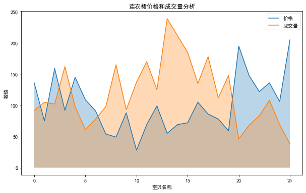
第八题

import pandas as pd
import matplotlib.pyplot as plt

# 读取数据
data = pd.read_excel(r'C:\Users\XXGC\Desktop\任务8 商品定价分析-素材8.xlsm')
df = pd.DataFrame(data)

# 绘制价格和成交量分析图
plt.figure(figsize=(10, 6))
plt.plot(prices, label="价格")
plt.plot(volumes, label="成交量")
plt.xlabel('价格（元）')
plt.ylabel('成交量（件）')
plt.title('连衣裙价格和成交量分析')
plt.title("连衣裙价格和成交量分析")
plt.xlabel("宝贝名称")
plt.ylabel("数值")
plt.fill_between(prices.index, prices, alpha=0.3)
plt.fill_between(volumes.index, volumes, alpha=0.3)

plt.legend()
plt.show()