


实验内容
算法实现:
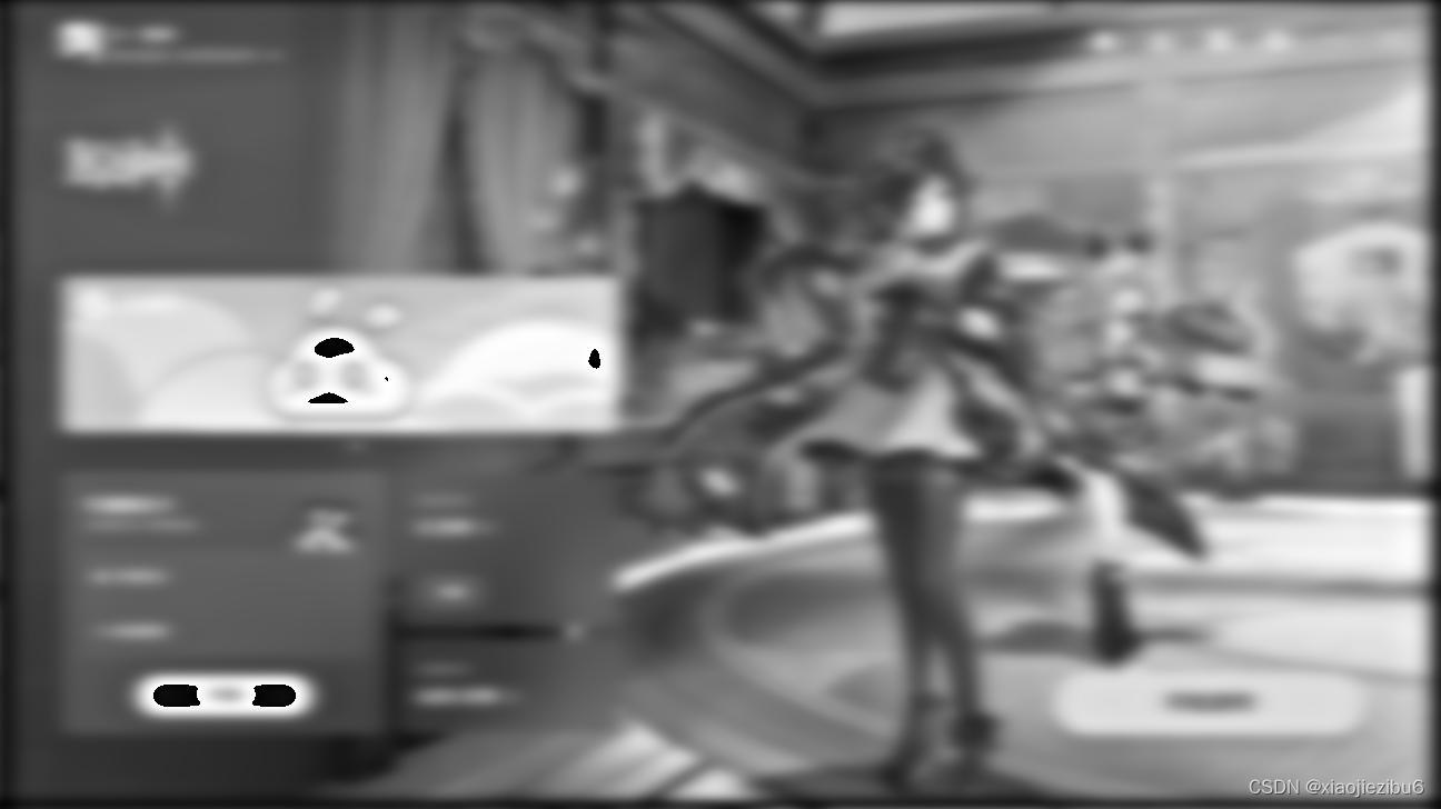
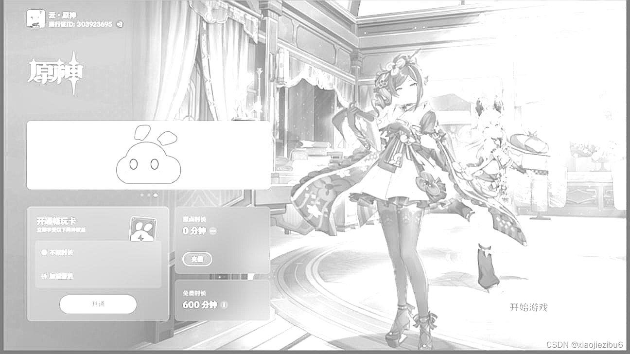
1.利用两个低通邻域平均模板(3×3 和 9×9)对一幅图像进行平滑,验证模板尺寸对 图像的模糊效果的影响。
代码展示:我们定义了一个卷积函数,传入图像数据和卷积核。随后读取图像信息,并定义两个卷积核的尺寸;随后调用先前定义的卷积函数,传入我们读取的图像数据和卷积核;最后将处理好的图像保存到本地并打印。因为运算量有点大,本人的笔记本年代有点久了,现跑代码要十几秒,所以加了一个保存的功能。
import numpy as np
from PIL import Image

def convolve(img, kernel):
    height, width = img.shape
    k_height, k_width = kernel.shape
    pad_h, pad_w = k_height // 2, k_width // 2

    # 对图像进行边缘填充
    padded_img = np.pad(img, ((pad_h, pad_h), (pad_w, pad_w)), mode='edge')

    # 创建输出图像
    output_img = np.zeros_like(img, dtype=np.float32)

    # 卷积操作
    for i in range(height):
        for j in range(width):
            roi = padded_img[i:i+k_height, j:j+k_width]
            output_img[i, j] = np.sum(roi * kernel)

    return output_img.astype(np.uint8)

# 读取图像
img = Image.open('image.jpg').convert('L')
img_array = np.array(img)

# 定义两个低通邻域平均模板
kernel_3x3 = np.ones((3, 3), np.float32) / 9
kernel_9x9 = np.ones((9, 9), np.float32) / 81

# 使用3x3模板进行平滑
smoothed_3x3 = convolve(img_array, kernel_3x3)

# 使用9x9模板进行平滑
smoothed_9x9 = convolve(img_array, kernel_9x9)

# 将平滑后的图像保存到本地
Image.fromarray(smoothed_3x3).save('smoothed_3x3.jpg')
Image.fromarray(smoothed_9x9).save('smoothed_9x9.jpg')

# 显示原图和平滑后的图像
Image.fromarray(img_array).show(title='Original')
Image.fromarray(smoothed_3x3).show(title='Smoothed (3x3)')
Image.fromarray(smoothed_9x9).show(title='Smoothed (9x9)')
这里展示一下代码的效果


可以发现,卷积核越大,平滑处理的效果越好,图像越模糊,消除的噪声越多,相应的损失的细节也越多。
2.利用一个低通模板对一幅含噪图像(Gauss 白噪声)进行滤波,检验两种滤波模板 (分别使用一个 5×5 的线性邻域平均模板和一个非线性模板 5×5 中值滤波器)对噪声的滤波效果。
代码展示:
由于题目要求是对"含噪图像(Gauss 白噪声)"进行处理,所以我们首先需要对图像进行加入高斯白噪声。
import numpy as np
from PIL import Image
import matplotlib.pyplot as plt

def add_gaussian_noise(image, mean=0, std=25):
    """
    在图像上添加高斯噪声
    :param image: PIL图像对象
    :param mean: 噪声的平均值
    :param std: 噪声的标准差
    :return: 含噪声的图像
    """
    image_np = np.array(image)
    # 生成和图像大小一致的高斯噪声
    noise = np.random.normal(mean, std, image_np.shape)
    # 将噪声添加到图像上
    noisy_image_np = image_np + noise
    # 确保结果仍然在合法的像素范围内
    noisy_image_np_clipped = np.clip(noisy_image_np, 0, 255)
    # 将结果从numpy数组转换回PIL图像
    noisy_image = Image.fromarray(np.uint8(noisy_image_np_clipped))
    return noisy_image

# 读取图像
image_path = 'image.jpg'
image = Image.open(image_path)

# 添加高斯噪声
noisy_image = add_gaussian_noise(image)

# 显示原图与含噪图像
plt.figure(figsize=(10, 5))
plt.subplot(1, 2, 1)
plt.imshow(image)
plt.title('Original Image')
plt.axis('off')

plt.subplot(1, 2, 2)
plt.imshow(noisy_image)
plt.title('Image with Gaussian Noise')
plt.axis('off')

plt.show()

# 如果需要,保存含噪图像
noisy_image_path = 'noisy_image.jpg'
noisy_image.save(noisy_image_path)
随后我们会得到这样子的图像,看起来锐化效果比较明显。

随后我们将处理后的噪声图像作为下文的输入图片,进行低通滤波。
from PIL import Image


def load_image(image_path):
    """加载图像,返回一个PIL图像对象"""
    return Image.open(image_path)


def save_image(image, output_path):
    """保存PIL图像对象到文件"""
    image.save(output_path)


def image_to_list(image):
    """将PIL图像转换为RGB值的三维列表"""
    pixels = list(image.getdata())
    w, h = image.size
    return [pixels[i * w:(i + 1) * w] for i in range(h)]


def list_to_image(pixels):
    """将RGB值的三维列表转换回PIL图像对象"""
    # 修正
    corrected_pixels = [[(0, 0, 0) if pixel is None else tuple(pixel) for pixel in row] for row in pixels]

    w, h = len(pixels[0]), len(pixels)
    # 创建一个新图像
    image = Image.new('RGB', (w, h))
    flat_list = [item for sublist in corrected_pixels for item in sublist]
    # 将扁平化的列表数据放入图像
    image.putdata(flat_list)
    return image


def apply_mean_filter(image):
    height = len(image)
    width = len(image[0])
    filtered_image = [[None for _ in range(width)] for _ in range(height)]

    for row in range(2, height - 2):
        for col in range(2, width - 2):
            for channel in range(3):
                sum_val = 0
                for i in range(-2, 3):
                    for j in range(-2, 3):
                        sum_val += image[row + i][col + j][channel]
                mean_val = sum_val / 25

                # 更改此处
                filtered_image[row][col] = filtered_image[row][col] or [0, 0, 0]
                filtered_image[row][col][channel] = int(mean_val)

    # 修改每个像素为元组
    for row in range(height):
        for col in range(width):
            if filtered_image[row][col] is not None:
                filtered_image[row][col] = tuple(filtered_image[row][col])

    return filtered_image


def apply_median_filter(image):
    height = len(image)
    width = len(image[0])
    filtered_image = [[None for _ in range(width)] for _ in range(height)]

    for row in range(2, height - 2):
        for col in range(2, width - 2):
            for channel in range(3):
                neighbors = []
                for i in range(-2, 3):
                    for j in range(-2, 3):
                        neighbors.append(image[row + i][col + j][channel])
                neighbors.sort()
                median_val = neighbors[12]

                # 更改此处
                filtered_image[row][col] = filtered_image[row][col] or [0, 0, 0]
                filtered_image[row][col][channel] = median_val

    # 修改每个像素为元组
    for row in range(height):
        for col in range(width):
            if filtered_image[row][col] is not None:
                filtered_image[row][col] = tuple(filtered_image[row][col])

    return filtered_image


# 主程序逻辑
if __name__ == "__main__":
    image_path = "image.jpg"  # 替换为你的图片路径
    output_path_mean = "output_mean.jpg"  # 替换为输出路径
    output_path_median = "output_median.jpg"  # 替换为输出路径

    # 加载图像
    image = load_image(image_path)

    # 转换为可操作的列表
    pixels = image_to_list(image)

    # 应用两种滤波器
    pixels_mean = apply_mean_filter(pixels)
    pixels_median = apply_median_filter(pixels)

    # 转换回PIL图像并保存
    image_mean = list_to_image(pixels_mean)
    save_image(image_mean, output_path_mean)

    image_median = list_to_image(pixels_median)
    save_image(image_median, output_path_median)
处理效果是这样的。


3.利用一个低通模板对一幅含噪图像(椒盐噪声)进行滤波,检验两种滤波模板(分别使用一个 5×5 的线性邻域平均模板和一个非线性模板 5×5 中值滤波器)对噪声的滤波效果。
代码展示:
类似第2题,我们首先对图像进行加入椒盐噪声处理。
import numpy as np
from PIL import Image
import matplotlib.pyplot as plt

def add_salt_and_pepper_noise(image, salt_prob=0.01, pepper_prob=0.01):
    """
    在图像上添加椒盐噪声
    :param image: PIL图像对象
    :param salt_prob: 添加盐的概率(白色像素)
    :param pepper_prob: 添加胡椒的概率(黑色像素)
    :return: 含噪声的图像
    """
    image_np = np.array(image)
    # 随机生成噪声
    noise = np.random.rand(*image_np.shape[:2])
    # 添加盐噪声
    image_np[noise < salt_prob] = 255
    # 添加胡椒噪声
    image_np[noise > 1 - pepper_prob] = 0
    # 将numpy数组转换回PIL图像
    noisy_image = Image.fromarray(image_np)
    return noisy_image

# 读取图像
image_path = 'image.jpg'  # 修改为你的图片路径
image = Image.open(image_path)

# 添加椒盐噪声
noisy_image = add_salt_and_pepper_noise(image, salt_prob=0.01, pepper_prob=0.01)

# 显示原图与含噪图像
plt.figure(figsize=(10, 5))
plt.subplot(1, 2, 1)
plt.imshow(image)
plt.title('Original Image')
plt.axis('off')

plt.subplot(1, 2, 2)
plt.imshow(noisy_image)
plt.title('Image with Salt and Pepper Noise')
plt.axis('off')

plt.show()

# 如果需要,保存含噪图像
noisy_image_path = 'impulse_noise_image.jpg'  # 修改为你希望保存的路径
noisy_image.save(noisy_image_path)

接着以此作为输入进行滤波
from PIL import Image

def load_image(image_path):
    """加载图像,返回一个PIL图像对象"""
    return Image.open(image_path)

def save_image(image, output_path):
    """保存PIL图像对象到文件"""
    image.save(output_path)

def image_to_list(image):
    """将PIL图像转换为RGB值的三维列表"""
    pixels = list(image.getdata())
    w, h = image.size
    return [pixels[i * w:(i + 1) * w] for i in range(h)]


def list_to_image(pixels):
    """将RGB值的三维列表转换回PIL图像对象"""
    w, h = len(pixels[0]), len(pixels)
    # 创建一个新图像
    image = Image.new('RGB', (w, h))
    # 确保pixels中的每个项都是元组
    flat_list = [tuple(item) if isinstance(item, list) else item for sublist in pixels for item in sublist]

    # Debugging helper: 检查flat_list中的项是否都符合预期格式
    for item in flat_list:
        if not isinstance(item, tuple) or not len(item) == 3:
            print(f"Invalid item found: {item}")
            raise ValueError("All items in `flat_list` must be tuples of length 3.")

    # 将扁平化的列表数据放入图像
    image.putdata(flat_list)
    return image


def apply_mean_filter(image):
    height = len(image)
    width = len(image[0])
    filtered_image = [[[0, 0, 0] for _ in range(width)] for _ in range(height)]

    # 均值滤波器的逻辑...
    # 确保滤波器逻辑对所有需要处理的像素进行了适当的处理
    for row in range(2, height - 2):
        for col in range(2, width - 2):
            for channel in range(3):
                sum_val = 0
                for i in range(-2, 3):
                    for j in range(-2, 3):
                        sum_val += image[row + i][col + j][channel]
                mean_val = sum_val / 25

                # 更改此处
                filtered_image[row][col] = filtered_image[row][col] or [0, 0, 0]
                filtered_image[row][col][channel] = int(mean_val)

    # 修改每个像素为元组
    for row in range(height):
        for col in range(width):
            if filtered_image[row][col] is not None:
                filtered_image[row][col] = tuple(filtered_image[row][col])

    return filtered_image

def apply_median_filter(image):
    height = len(image)
    width = len(image[0])
    filtered_image = [[[0, 0, 0] for _ in range(width)] for _ in range(height)]

    # 中值滤波器的逻辑...
    # 确保滤波器逻辑对所有需要处理的像素进行了适当的处理
    for row in range(2, height - 2):
        for col in range(2, width - 2):
            for channel in range(3):
                neighbors = []
                for i in range(-2, 3):
                    for j in range(-2, 3):
                        neighbors.append(image[row + i][col + j][channel])
                neighbors.sort()
                median_val = neighbors[12]

                # 更改此处
                filtered_image[row][col] = filtered_image[row][col] or [0, 0, 0]
                filtered_image[row][col][channel] = median_val

    # 修改每个像素为元组
    for row in range(height):
        for col in range(width):
            if filtered_image[row][col] is not None:
                filtered_image[row][col] = tuple(filtered_image[row][col])

    return filtered_image

# 主程序逻辑
if __name__ == "__main__":
    image_path = "impulse_noise_image.jpg"  # 请替换为你的图片路径
    output_path_mean = "output_mean.jpg"  # 输出路径
    output_path_median = "output_median.jpg"  # 输出路径

    # 加载图像
    image = load_image(image_path)

    # 转换为可操作的列表
    pixels = image_to_list(image)

    # 应用两种滤波器
    pixels_mean = apply_mean_filter(pixels)
    pixels_median = apply_median_filter(pixels)

    # 转换回PIL图像并保存
    image_mean = list_to_image(pixels_mean)
    save_image(image_mean, output_path_mean)

    image_median = list_to_image(pixels_median)
    save_image(image_median, output_path_median)


4.对图像一幅图像加入椒盐噪声后,实现 Butterworth 低通滤波。(频域处理,可选做)
由于是对含椒盐噪声的图像进行处理,所以这里要拿第3题中的含噪图片impulse_noise_image.jpg来作为输入,但是实测发现如果拿原图image.jpg处理似乎也差不多。
import numpy as np
from PIL import Image
import matplotlib.pyplot as plt


# 读取图像并转换为灰度
def load_image(image_path):
    image = Image.open(image_path)
    image = image.convert('L')  # 转换为灰度图像
    return np.asarray(image)


# 实现Butterworth低通滤波器
def butterworth_lowpass_filter(image, cutoff_freq, order):
    h, w = image.shape
    Y, X = np.ogrid[:h, :w]
    distance_center = np.sqrt((X - w / 2) ** 2 + (Y - h / 2) ** 2)
    butterworth_filter = 1 / (1 + (distance_center / cutoff_freq) ** (2 * order))
    return butterworth_filter


# 应用滤波器
def apply_filter(image, filter):
    dft_image = np.fft.fft2(image)
    dft_image_shifted = np.fft.fftshift(dft_image)

    filtered_dft = dft_image_shifted * filter
    filtered_dft_shifted_back = np.fft.ifftshift(filtered_dft)
    filtered_image = np.fft.ifft2(filtered_dft_shifted_back)

    return np.abs(filtered_image)


# 假设 load_image, butterworth_lowpass_filter, apply_filter 函数已经被定义

def save_image(np_image, output_path):
    """保存NumPy数组为图像"""
    # 将NumPy数组转换为PIL图像
    pil_image = Image.fromarray(np.uint8(np_image))
    # 保存图像
    pil_image.save(output_path)
    print(f"Image saved to {output_path}")

if __name__ == "__main__":
    # 步骤 1
    image_path = "impulse_noise_image.jpg"  # 请替换为你的文件路径
    image = load_image(image_path)

    # 步骤 2 和步骤 3
    cutoff_frequency = 30  # 截止频率,可根据实际情况调整
    order = 2  # 滤波器阶数,可根据实际情况调整
    bw_filter = butterworth_lowpass_filter(image, cutoff_frequency, order)

    # 步骤 4
    filtered_image = apply_filter(image, bw_filter)

    # 显示图像
    plt.figure(figsize=(12, 6))
    plt.subplot(121), plt.imshow(image, cmap='gray')
    plt.title('Original Image'), plt.xticks([]), plt.yticks([])
    plt.subplot(122), plt.imshow(filtered_image, cmap='gray')
    plt.title('Filtered Image'), plt.xticks([]), plt.yticks([])
    plt.show()

    # 保存处理后的图像
    output_path = "filtered_image.jpg"  # 指定保存路径
    save_image(filtered_image, output_path)
51.选用一幅经过低通滤波器滤波处理的模糊图像,利用 Laplacian 算子对其进行锐化处理。
这里要求对低通滤波器滤波处理后的模糊图像进行处理,所以可以直接拿第4题的输出图片filtered_image.jpg作为本题的输入。
代码展示:
import numpy as np
from PIL import Image


def load_image(image_path):
    """加载图像,返回一个Numpy数组"""
    image = Image.open(image_path).convert('L')  # 转换为灰度图像
    return np.array(image)


def save_image(image_array, output_path):
    """将Numpy数组保存为图像"""
    image = Image.fromarray(np.uint8(image_array))
    image.save(output_path)


def laplacian_sharpen(image_array):
    """使用Laplacian算子对图像进行锐化处理"""
    kernel = np.array([[-1, -1, -1],
                       [-1, 8, -1],
                       [-1, -1, -1]])  # Laplacian核
    height, width = image_array.shape
    # 创建一个和原图像相同大小的零数组(边缘不处理,故稍小)
    result_array = np.zeros((height, width), dtype=np.float32)

    # 卷积操作
    for i in range(1, height - 1):
        for j in range(1, width - 1):
            result_array[i, j] = np.sum(image_array[i - 1:i + 2, j - 1:j + 2] * kernel)

    # 归一化到 0-255
    result_array = (result_array - np.min(result_array)) / (np.max(result_array) - np.min(result_array)) * 255

    # 将锐化后的图像与原图像叠加
    sharpened_image = image_array + result_array
    sharpened_image = np.clip(sharpened_image, 0, 255)  # 限制值的范围在0到255之间

    return sharpened_image


if __name__ == "__main__":
    image_path = "../mean_filtered_image.jpg"  # 输入图像路径
    output_path = "sharpened_image.jpg"  # 输出图像路径

    # 加载图像
    image_array = load_image(image_path)

    # 使用Laplacian算子对图像进行锐化处理
    sharpened_image_array = laplacian_sharpen(image_array)

    # 保存处理后的图像
    save_image(sharpened_image_array, output_path)

    print("Image processing completed and saved to", output_path)
处理效果
52.选择一个经过低通滤波器滤波的模糊图像,利用 sobel 和 prewitt 算子边缘增强高通滤 波器(模板)对其进行高通滤波图像边缘增强,验证模板的滤波效果。
同样,将第4题的输出图片filtered_image.jpg作为本题的输入。
代码展示:
import numpy as np
from PIL import Image
import matplotlib.pyplot as plt


def load_image(image_path):
    """加载图像,返回灰度图像的Numpy数组"""
    return np.array(Image.open(image_path).convert('L'))


def save_image(image_array, output_path):
    """将Numpy数组保存为图像"""
    Image.fromarray(np.uint8(image_array)).save(output_path)


def apply_filter(image, kernel):
    """应用给定的核对图像进行卷积"""
    pad_width = kernel.shape[0] // 2
    padded_image = np.pad(image, pad_width, mode='edge')
    filtered_image = np.zeros_like(image)

    for i in range(image.shape[0]):
        for j in range(image.shape[1]):
            filtered_image[i, j] = np.sum(
                padded_image[i:i + kernel.shape[0], j:j + kernel.shape[1]] * kernel)

    return filtered_image


def normalize_image(image):
    """将图像数据归一化到[0, 255]范围内"""
    normalized_image = 255 * (image - np.min(image)) / (np.max(image) - np.min(image))
    return normalized_image


def sobel_prewitt_edge_enhancement(image_path, output_sobel_path, output_prewitt_path):
    """使用Sobel和Prewitt算子进行边缘增强"""
    # Sobel算子
    sobel_x = np.array([[-1, 0, 1], [-2, 0, 2], [-1, 0, 1]])
    sobel_y = np.array([[-1, -2, -1], [0, 0, 0], [1, 2, 1]])

    # Prewitt算子
    prewitt_x = np.array([[-1, 0, 1], [-1, 0, 1], [-1, 0, 1]])
    prewitt_y = np.array([[-1, -1, -1], [0, 0, 0], [1, 1, 1]])

    # 加载图像
    image = load_image(image_path)

    # 应用Sobel算子
    sobel_filtered_image = np.sqrt(apply_filter(image, sobel_x) ** 2 + apply_filter(image, sobel_y) ** 2)
    sobel_filtered_image_normalized = normalize_image(sobel_filtered_image)

    # 应用Prewitt算子
    prewitt_filtered_image = np.sqrt(apply_filter(image, prewitt_x) ** 2 + apply_filter(image, prewitt_y) ** 2)
    prewitt_filtered_image_normalized = normalize_image(prewitt_filtered_image)

    # 保存处理后的图像
    save_image(sobel_filtered_image_normalized, output_sobel_path)
    save_image(prewitt_filtered_image_normalized, output_prewitt_path)

    # 使用matplotlib显示结果
    plt.figure(figsize=(12, 6))
    plt.subplot(1, 2, 1)
    plt.imshow(sobel_filtered_image_normalized, cmap='gray')
    plt.title('Sobel Filtered')
    plt.axis('off')

    plt.subplot(1, 2, 2)
    plt.imshow(prewitt_filtered_image_normalized, cmap='gray')
    plt.title('Prewitt Filtered')
    plt.axis('off')

    plt.show()


if __name__ == "__main__":
    image_path = "../mean_filtered_image.jpg"  # 输入图像的路径
    output_sobel_path = "sobel_filtered_image.jpg"  # Sobel算子处理后的输出路径
    output_prewitt_path = "prewitt_filtered_image.jpg"  # Prewitt算子处理后的输出路径

    sobel_prewitt_edge_enhancement(image_path, output_sobel_path, output_prewitt_path)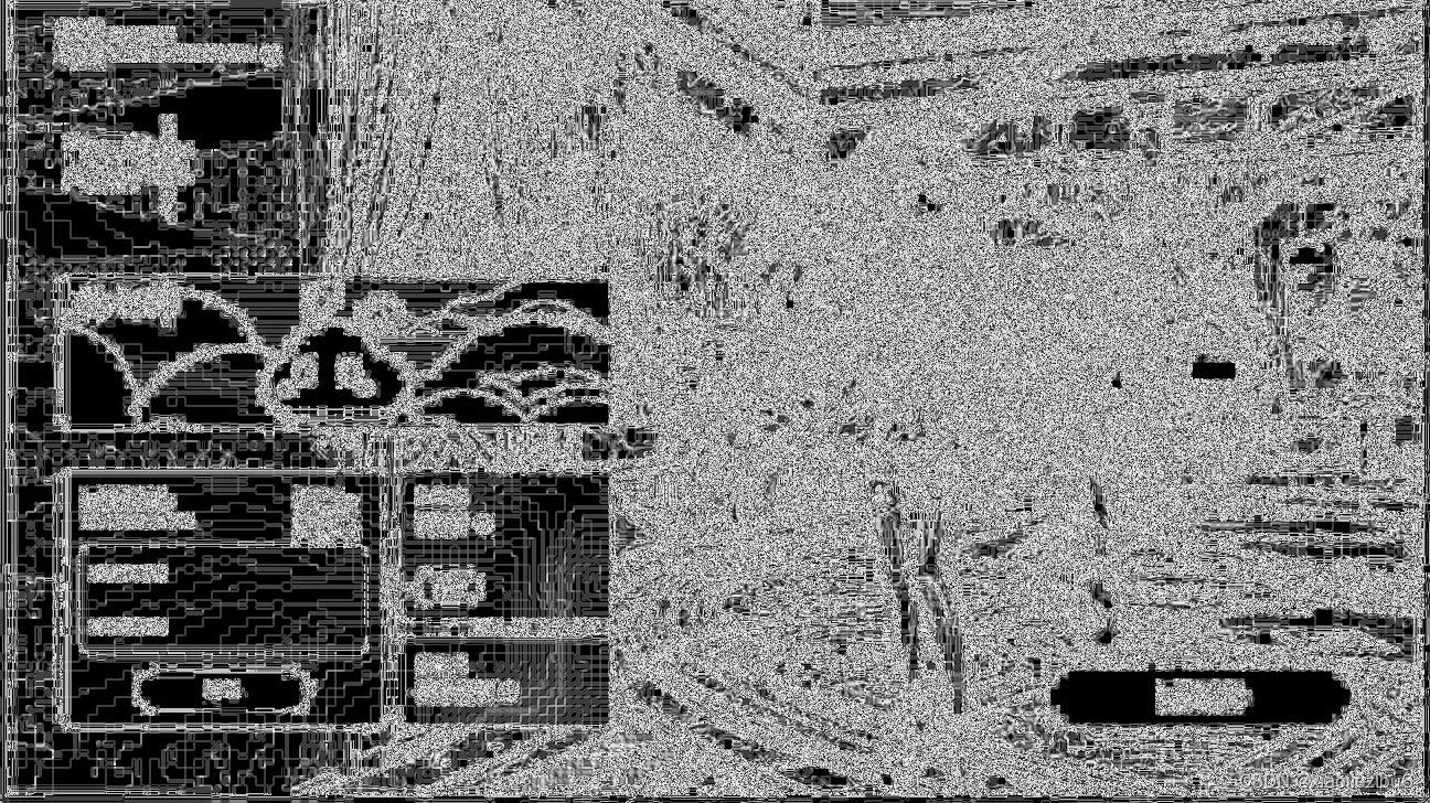
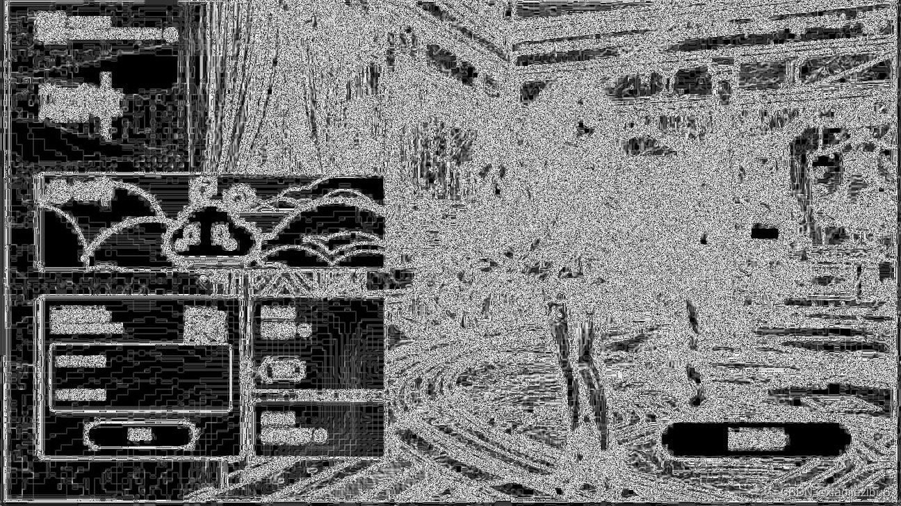
6.选择一幅灰度图像分别利用 一阶Sobel算子和二阶Laplacian算子对其进行边缘检测, 验证检测效果。
灰度处理比较好处理,我们可以在读取图片的时候直接转换,所以这里就不用两个代码了。
import numpy as np
from PIL import Image
import matplotlib.pyplot as plt


def load_image(image_path):
    """加载图像,并转换成灰度图像"""
    return np.array(Image.open(image_path).convert('L'))


def save_image(image_array, output_path):
    """将Numpy数组保存为图像,确保输入为uint8类型"""
    Image.fromarray(image_array).save(output_path)


def apply_filter(image, kernel):
    """对图像使用指定的核进行卷积操作"""
    height, width = image.shape
    kernel_height, kernel_width = kernel.shape
    pad_height, pad_width = kernel_height // 2, kernel_width // 2
    padded_image = np.pad(image, ((pad_height, pad_height), (pad_width, pad_width)), mode='constant', constant_values=0)

    filtered_image = np.zeros((height, width))
    for i in range(height):
        for j in range(width):
            filtered_image[i, j] = np.sum(padded_image[i:i + kernel_height, j:j + kernel_width] * kernel)
    return filtered_image


def normalize_image(image):
    """归一化图像数据到0-255范围,并将其转换为uint8类型"""
    norm_image = 255 * (image - np.min(image)) / (np.max(image) - np.min(image))
    return norm_image.astype(np.uint8)


if __name__ == "__main__":
    image_path = "../image.jpg"  # 请更改为您的图片路径
    output_sobel_path = "sobel_edge_detection.jpg"
    output_laplacian_path = "laplacian_edge_detection.jpg"

    # Sobel算子
    sobel_x = np.array([[-1, 0, 1], [-2, 0, 2], [-1, 0, 1]])
    sobel_y = np.array([[-1, -2, -1], [0, 0, 0], [1, 2, 1]])
    # Laplacian算子
    laplacian = np.array([[0, 1, 0], [1, -4, 1], [0, 1, 0]])

    image = load_image(image_path)

    sobel_image = apply_filter(image, sobel_x) + apply_filter(image, sobel_y)
    laplacian_image = apply_filter(image, laplacian)

    # 这里直接进行归一化处理
    sobel_image_normalized = normalize_image(sobel_image)
    laplacian_image_normalized = normalize_image(laplacian_image)

    # 显示图像
    plt.figure(figsize=(12, 6))
    plt.subplot(1, 2, 1)
    plt.imshow(sobel_image_normalized, cmap='gray')
    plt.title('Sobel Edge Detection')
    plt.axis('off')

    plt.subplot(1, 2, 2)
    plt.imshow(laplacian_image_normalized, cmap='gray')
    plt.title('Laplacian Edge Detection')
    plt.axis('off')

    plt.show()

    # 保存图像
    save_image(sobel_image_normalized, output_sobel_path)
    save_image(laplacian_image_normalized, output_laplacian_path)

当做到这里的时候,我突然觉得数字图像处理真的是很牛。sobel_edge_detection.jpg非常的有浮雕的质感,而laplacian_edge_detection.jpg似乎可以应用到线稿?(无端联想)
7.对一幅图像实现 Butterworth 高通滤波。(高频提升滤波法。可选做)
代码展示:
import numpy as np
from PIL import Image
import matplotlib.pyplot as plt


def load_image(image_path):
    """加载图像并转换为灰度图像"""
    return np.array(Image.open(image_path).convert('L'))


def save_image(image_array, output_path):
    """保存图像数组为文件"""
    Image.fromarray(np.uint8(image_array)).save(output_path)


# 避免除以0操作
def butterworth_highpass_filter(d0, shape, n):
    """创建Butterworth高通滤波器的频域滤波窗口"""
    P, Q = shape
    D0 = d0
    H = np.zeros((P, Q))
    for u in range(P):
        for v in range(Q):
            D = np.sqrt((u - P/2)**2 + (v - Q/2)**2)
            if D == 0:  # 避免除以零的错误
                H[u, v] = 0
            else:
                H[u, v] = 1 / (1 + (D0/D)**(2*n))
    return H


def apply_butterworth_highpass_filter(image_path):
    """应用Butterworth高通滤波器并显示处理后的图像"""
    image = load_image(image_path)
    d0 = 30  # 截止频率
    n = 2  # Butterworth滤波器的阶数

    # 转换到频域
    f = np.fft.fftshift(np.fft.fft2(image))

    # 创建滤波器
    H = butterworth_highpass_filter(d0, image.shape, n)

    # 应用滤波器并转换回空间域
    filtered_image = np.real(np.fft.ifft2(np.fft.ifftshift(f * H)))

    # 归一化到[0, 255]
    filtered_image = np.clip(filtered_image, 0, 255)

    # 显示原始和处理后的图像
    plt.figure(figsize=(12, 6))
    plt.subplot(1, 2, 1)
    plt.imshow(image, cmap='gray')
    plt.title('Original Image')
    plt.axis('off')

    plt.subplot(1, 2, 2)
    plt.imshow(filtered_image, cmap='gray')
    plt.title('Butterworth Highpass Filtered Image')
    plt.axis('off')

    plt.show()

    # 保存处理后的图像
    save_image(filtered_image, 'butterworth_highpass_filtered_image.jpg')


if __name__ == "__main__":
    image_path = "../image.jpg"  # 修改为你的图像路径
    apply_butterworth_highpass_filter(image_path)
这个图像处理的效果黑黢黢的,有种说不出来的感觉。
总结
至此,数字图像处理的实验四就做完了。有的算法处理的效果还是很让人惊艳的,就比如一阶Sobel算子和二阶Laplacian算子,给人很舒服的质感。由于成稿匆忙,所以解释的不多,如果有时间考虑再详细解释一下。最后希望能帮到大家。.
链接:https://pan.quark.cn/s/ff3b2b494029
hhttps://pan.quark.cn/s/ff3b2b494029
直接点击跳转慢可以手动复制到浏览器打开。
(我发现很多平台都热衷于检测链接,但是无疑增加了用户的时间成本,刚刚实测发现长按竟然无法复制,链接直接悬浮了,所以又写了一个链接,只用把开头的h去掉即可。


 9421
9421


 被折叠的 条评论
为什么被折叠?
被折叠的 条评论
为什么被折叠?
 到【灌水乐园】发言


