Weather Data Analysis Example:Part 3a

Part 3a: Plotting with ggplot2

We will start off this first section of Part 3 with a brief introduction of the plotting system ggplot2. Then, with the attention focused mainly on the syntax, we will create a few graphs, based  on the weather data we have prepared previously.

Next, in Part 3b, where we will be doing actual EDA, specific visualisations using ggplot2 will be developed, in order to address the following question: Are there any good predictors, in our data, for the occurrence of rain on a given day?

Lastly, in Part 4, we will use Machine Learning algorithms to check to which extent rain can be predicted based on the variables available to us.

But for now, let's see what this ggplot2 system is all about and create a few nice looking figures.

 

The concept of ggplot2

The R package ggplot2, created by Hadley Wickham, is an implementation of Leland Wilkinson's Grammar of Graphics, which is a systematic approach to describe the components of a graphic. In maintenance mode (i.e., no active development) since February 2014, ggplot2 it is the most downloaded R package of all time.

In ggplot2, the graphics are constructed out of layers. The data being plotted, coordinate system, scales, facets, labels and annotations, are all examples of layers. This means that any graphic, regardless of how complex it might be, can be built from scratch by adding simple layers, one after another, until one is satisfied with the result. Each layer of the plot may have several different components, such as: data, aesthetics (mapping), statistics (stats), etc. Besides the data (i.e., the R data frame from where we want to plot something), aesthetics and geometries are particularly important, and we should make a clear distinction between them:

• Aesthetics are visual elements mapped to data; the most common aesthetic attributes are the x and y values, colour, size, and shape;
• Geometries are the actual elements used to plot the data, for example: point, line, bar, map, etc.

So, what does this mean in practice? Suppose we want to draw a scatter plot to show the relationship between the minimum and maximum temperatures on each day, controlling for the season of the year using colour (good for categorical variables), and the rain using size (good for continuous variables). We would map the aesthetics x, y, colour and size to the respective data variables, and then draw the actual graphic using a geometry - in this case, geom_point().

Here are some important aspects to have in mind:

• Not all aesthetics of a certain geometry have to be mapped by the user, only the required ones. For example, in the case above we didn't map the shape of the point, and therefore the system would use the default value (circle); it should be obvious, however, that x and y have no defaults and therefore need to be either mapped or set;
• Some aesthetics are specific of certain geometries - for instance, ymin and ymax are required aesthetics for geom_errorbar(), but don't make sense in the context of geom_point();
• We can map an aesthetic to data (for example, colour = season), but we can also set it to a constant value (for example, colour = "blue"). There are a few subtleties when writing the actual code to map or set an aesthetic, as we will see below.

 

 

The syntax of ggplot2

A basic graphic in ggplot2 consists of initializing an object with the function ggplot() and then add the geometry layer. 

• ggplot() - this function is always used first, and initializes a ggplot object. Here we should declare all the components that are intended to be common to all the subsequent layers. In general, these components are the data (the R data frame) and some of the aesthetics (mapping visual elements to data, via the aes() function). As an example:

ggplot(data = dataframe, aes(x = var1, y= var2, colour = var3, size = var4))

• geom_xxx() - this layer is added after ggplot() to actually draw the graphic.  If all the required aesthetics were already declared in ggplot(), it can be called without any arguments. If an aesthetic previously declared in ggplot() is also declared in the geom_xxx layer, the latter overwrites the former. This is also the place to map or set specific components specific to the layer. A few real examples from our weather data should make it clear:

# This draws a scatter plot where season controls the colour of the point

ggplot(data = weather, aes(x = l.temp, y= h.temp, colour = season) + geom_point()

# This draws a scatter plot but colour is now controlled by dir.wind (overwrites initial definition)

ggplot(data = weather, aes(x = l.temp, y= h.temp, colour = season) + geom_point(aes(colour=dir.wind))

# This sets the parameter colour to a constant instead of mapping it to data. This is outside aes()!

ggplot(data = weather, aes(x = h.temp, y= l.temp) + geom_point(colour = "blue")

# Mapping to data (aes) and setting to a constant inside the geom layer

ggplot(data = weather, aes(x = l.temp, y= h.temp) + geom_point(aes(size=rain), colour = "blue")

# This is a MISTAKE - mapping with aes() when intending to set an aesthetic. It will create a column in the data named "blue", which is not what we want.

ggplot(data = weather, aes(x = l.temp, y= h.temp) + geom_point(aes (colour = "blue"))

When learning the ggplot2 system, this is a probably a good way to make the process easier:

1. Decide what geom you need - go here, identify the geom best suited for your data, and then check which aesthetics it understands (both the required, that you will need to specify, and the optional ones, that more often than not are useful);
2. Initialize the plot with ggplot() and map the aesthetics that you intend to be common to all the subsequent layers (don't worry too much about this, you can always overwrite aesthetics if needed);
3. Make sure you understand if you want an aesthetic to be mapped to data or set to a constant. Only in the former the aes() function is used. 

Although aesthetics and geometries are probably the most important part of ggplot2, there are more layers/components that we will be using often, such as scales (both colour scales and axes-controlling ones), statistics, and faceting (this one surely in Part 3b). Now, let's make some plots using different geometries!

 

Plotting a time series - point geom with smoother curve

# Time series of average daily temperature, with smoother curve

ggplot(weather,aes(x = date,y = ave.temp)) +
  geom_point(colour = "blue") +
  geom_smooth(colour = "red",size = 1) +
  scale_y_continuous(limits = c(5,30), breaks = seq(5,30,5)) +
  ggtitle ("Daily average temperature") +
  xlab("Date") +  ylab ("Average Temperature ( ºC )")

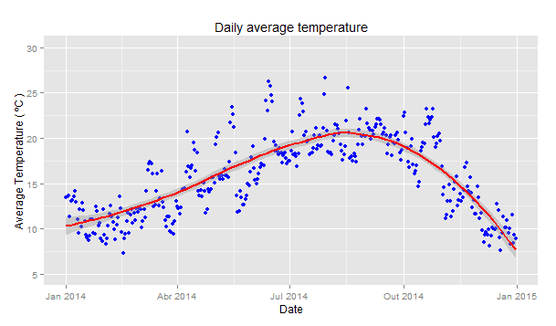
Instead of setting the colour to blue, we can map it to the value of the temperature itself, using the aes() function. Moreover, we can define the color gradient we want - in this case, I told that cold days should be blue and warm days red. I forced the gradient to go through green, and pure green should occur when the temperature is 16 ºC. There are many ways to work with colour, and it would be impossible for us to cover everything. 

# Same but with colour varying

ggplot(weather,aes(x = date,y = ave.temp)) + 
  geom_point(aes(colour = ave.temp)) +
  scale_colour_gradient2(low = "blue", mid = "green" , high = "red", midpoint = 16) + 
  geom_smooth(color = "red",size = 1) +
  scale_y_continuous(limits = c(5,30), breaks = seq(5,30,5)) +
  ggtitle ("Daily average temperature") +
  xlab("Date") +  ylab ("Average Temperature ( ºC )")

The smoother curve (technically a loess) drawn on the graphs above shows the typical pattern for a city in the northern hemisphere, i.e., higher temperatures in July (summer) and lower in January (winter).

 

 

Analysing the temperature by season - density geom

# Distribution of the average temperature by season - density plot

ggplot(weather,aes(x = ave.temp, colour = season)) +
  geom_density() +
  scale_x_continuous(limits = c(5,30), breaks = seq(5,30,5)) +
  ggtitle ("Temperature distribution by season") +
  xlab("Average temperature ( ºC )") +  ylab ("Probability")

 

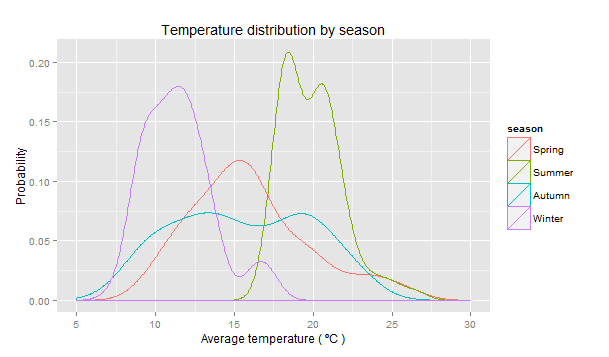
I find this graph interesting. Spring and autumn seasons are often seen as the transition from cold to warm and warm to cold days, respectively. The spread of their distributions reflect the high thermal amplitude of these seasons. On the other hand, winter and summer average temperatures are much more concentrated around a few values, and hence the peaks shown on the graph.

 

Analysing the temperature by month - violin geom with jittered points overlaid

# Label the months - Jan...Dec is better than 1...12

weather$month = factor(weather$month,
                       labels = c("Jan","Fev","Mar","Apr",
                                  "May","Jun","Jul","Aug","Sep",
                                  "Oct","Nov","Dec"))

# Distribution of the average temperature by month - violin plot,
# with a jittered point layer on top, and with size mapped to amount of rain

ggplot(weather,aes(x = month, y = ave.temp)) +
  geom_violin(fill = "orange") +
  geom_point(aes(size = rain), colour = "blue", position = "jitter") +
  ggtitle ("Temperature distribution by month") +
  xlab("Month") +  ylab ("Average temperature ( ºC )")

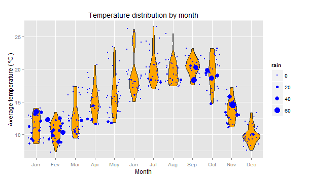
A violin plot is sort of a mixture of a box plot with a histogram (or even better, a rotated density plot). I also added a point layer on top (with jitter for better visualisation), in which the size of the circle is mapped to the continuous variable representing the amount of rain. As can be seen, there were several days in the autumn and winter of 2014 with over 60 mm of precipitation, which is more than enough to cause floods in some vulnerable zones. In subsequent parts, we will try to learn more about rain and its predictors, both with visualisation techniques and machine learning algorithms.

 

Analysing  the correlation between low and high temperatures

# Scatter plot of low vs high daily temperatures, with a smoother curve for each season

ggplot(weather,aes(x = l.temp, y = h.temp)) +
  geom_point(colour = "firebrick", alpha = 0.3) + 
  geom_smooth(aes(colour = season),se= F, size = 1.1) +
  ggtitle ("Daily low and high temperatures") +
  xlab("Daily low temperature ( ºC )") +  ylab ("Daily high temperature ( ºC )") 

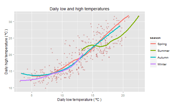
The scatter plot shows a positive correlation between the low and high temperatures for a given day, and it holds true regardless of the season of the year. This is a good example of a graphic where we set an aesthetic for one geom (point colour) and mapped an aesthetic for another (smoother curve colour).

 

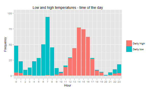
Distribution of low and high temperatures by the time of day

 

In this final example, we would like to plot the frequencies of two data series (i.e. two variables) on the same graph, namely, the lowest and highest daily temperatures against the hour when they occurred. The way these variables are represented in our data set is called wide data form, which is used, for instance, in MS Excel, but it is not the first choice in ggplot2, where the long data form is preferred.

Let's think a bit about this important, albeit theoretical, concept. When we plotted the violin graph before, did we have wide data (12 numerical variables, each one containing the temperatures for each month), or long data (1 numerical variable with all temperatures and 1 grouping variable with the month information)? Definitely the latter. This is exactly need what we need to do to our 2 temperature variables: create a grouping variable that, for each row, represents either a low temperature or a high temperature, and a numerical variable indicating the corresponding hour of the day. The example in the code below should help understanding this concept (for further information on this topic, please have a look at the tidy data article mentioned in Part 1 of this tutorial).

> # We will use the melt function from reshape2 to convert from wide to long form
> library(reshape2) 

> # select only the variables that are needed (day and temperatures) and assign to a new data frame
> temperatures <- weather[c("day.count","h.temp.hour","l.temp.hour")] 

> # Temperature variables in columns
> head(temperatures)
  day.count h.temp.hour l.temp.hour
1         1           0           1
2         2          11           8
3         3          14          21
4         4           2          11
5         5          13           2
6         6           0          20 

> dim(temperatures)
[1] 365   3 

> # The temperatures are molten into a single variable called l.h.temp 

> temperatures <- melt(temperatures,id.vars = "day.count",
                       variable.name = "l.h.temp", value.name = "hour")

> # See the difference?
> head(temperatures)
  day.count    l.h.temp hour
1         1 h.temp.hour    0
2         2 h.temp.hour   11
3         3 h.temp.hour   14
4         4 h.temp.hour    2
5         5 h.temp.hour   13
6         6 h.temp.hour    0 

> tail(temperatures)
    day.count    l.h.temp hour
725       360 l.temp.hour    7
726       361 l.temp.hour    4
727       362 l.temp.hour   23
728       363 l.temp.hour    8
729       364 l.temp.hour    5
730       365 l.temp.hour    8 

> # We now have twice the rows. Each day has an observation for low and high temperatures
> dim(temperatures)
[1] 730   3 

> # Needed to force the order of the factor's level
> temperatures$hour <- factor(temperatures$hour,levels=0:23)

# Now we can just fill the colour by the grouping variable to visualise the two distributions 
ggplot(temperatures) +
  geom_bar(aes(x = hour, fill = l.h.temp)) +
  scale_fill_discrete(name= "", labels = c("Daily high","Daily low")) +
  scale_y_continuous(limits = c(0,100)) +
  ggtitle ("Low and high temperatures - time of the day") +
  xlab("Hour") +  ylab ("Frequency")

The graph clearly shows with we know from experience: the daily lowest temperatures tend to occur early in the morning and the highest in the afternoon. But can you see those outliers in the distribution? There were a few days were the highest temperature was during the night, and a few others where the lowest was during the day. Can this somehow be correlated to rain? This is the kind of questions we will be exploring in Part 3b, where we will use EDA techniques (visualisations) to identify potential predictors for the occurrence of rain. Then, in Part 4, using data mining and machine learning algorithms, not only we will find the best predictors for rain (if any) and determine the accuracy of the models, but also the individual contribution of each variable in our data set.

More to come soon... stay tuned!