


Code: Julia
Introduction
History
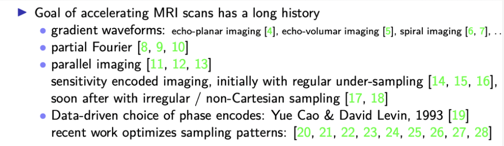
mri scans are slow because you collect
one point in case space at a time
basically and so there's been a long
history
of working on methods to try and
accelerate mri scans to make them more
affordable to make them more comfortable
for patients to reduce motion artifacts
and so on
and there's both hardware-based methods
for try to make them faster
as well as different ways of collecting
the case-based data
uh to to reduce how much time you spend
collecting that data
and using parallel imaging which we'll
talk about more later to to give us
additional information so that we can
collect fewer samples
in fact this has such a long history
that even back as far as 1993
people were working on data adaptive
methods
uh for choosing which locations in k
space
to sample and and there's been a very
recent
uh trend towards uh revisiting or really
digging in much more detail that topic
of of using training data to
choose the sampling patterns
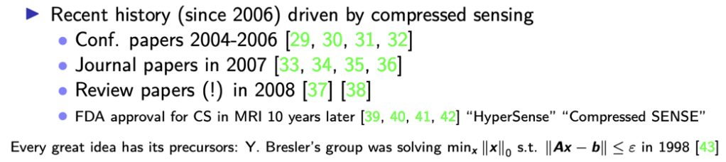
in the last 10 plus years compressed
sensing certainly has been a major theme
initially there were conference papers
in the 046 kind of time frame
leading to some journal paper shortly
after that and leading to review papers
right after that
and then finally in 2017 the fda
approved compressed sensing methods for
mri
and it's now all of the major
manufacturers have fda approved
compressed sensing methods that are used
to various degrees by the different
manufacturer systems
for clinical scan so this is a real
success story i think for the imaging
science community the applied math
community
that those contributions in sparsity
compressed sensing
uh have led to you know routine clinical
use
of that technology under various names
like compressed sense and hyper sense in
the field
uh again you know the the real focus on
this began
like i said 10 13 14 years ago but again
every good idea has its earlier
precursors and yorn brussels group at
illinois was solving sparsely
sparsity related problems even as far
back as 1998.
scope
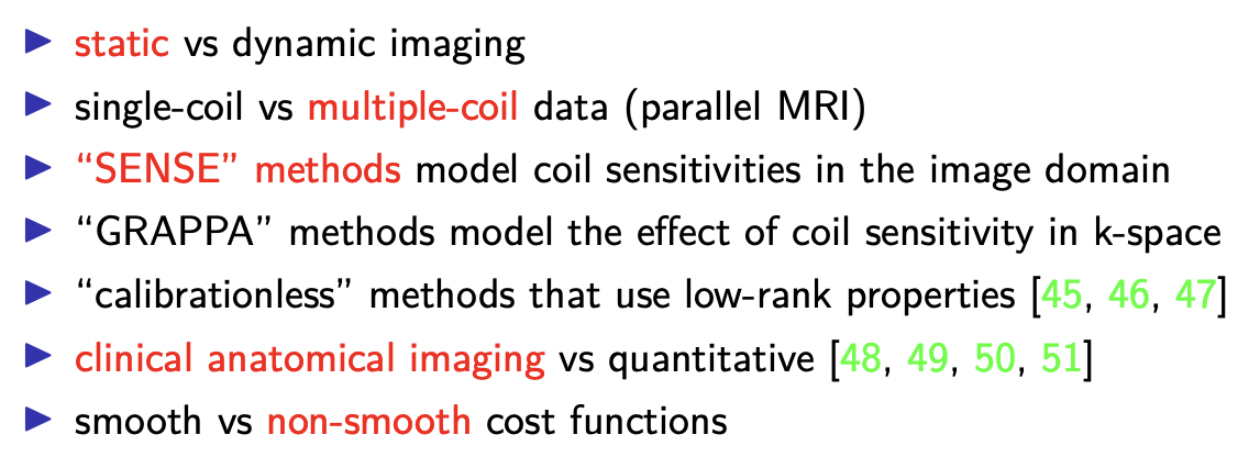
i want
to give you a sense of the scope of what
i'll be emphasizing
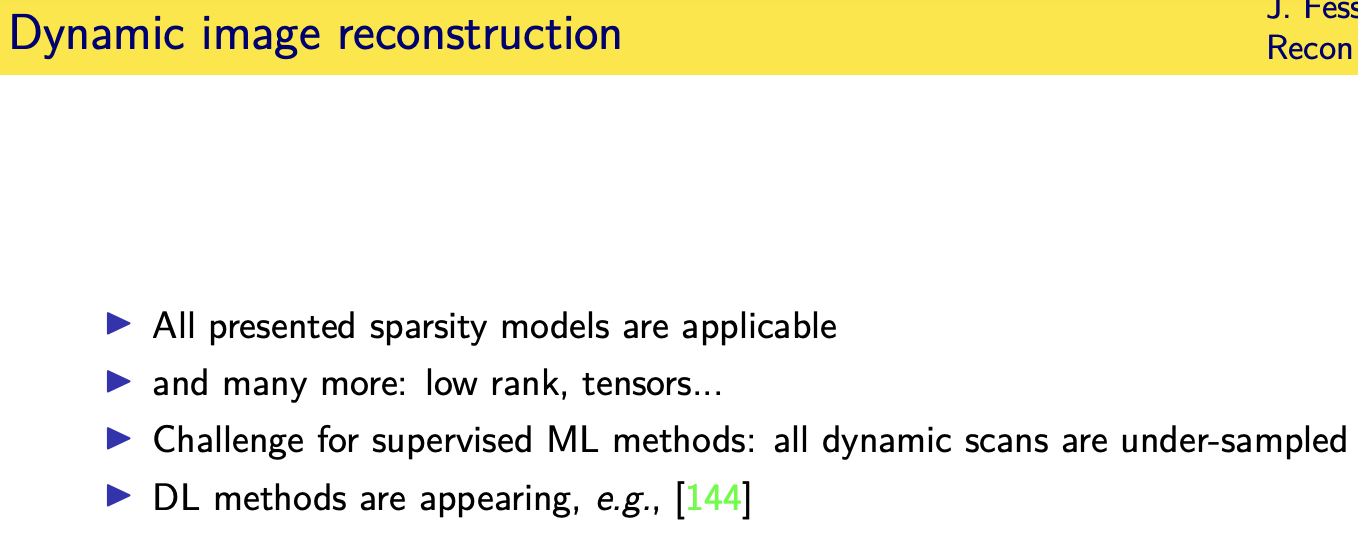
i'm going to focus on static imaging as
opposed to dynamic imaging there's a
whole other set of tools that are needed
for dynamic imaging and there's some
nice
survey papers on that in uh the i think
the january 2020 issue by tripoli
signal processing magazine if you're
interested in that broader scope
i'm going to focus on multiple coil or parallel mri data as opposed to single coil
because that's what all the vendors use today and i would argue that any
any submitted papers that consider single coil mri are not very interesting
anybody who's going to do advanced reconstruction methods
is going to be doing it with multi-coil
data so that would be my focus
for those of you are mri experts i'm
going to be focusing on sense methods
that model the coil sensitivities
there are another family of methods or
sometimes called grappa methods that
model them in k-space and i won't be
giving them as much focus
there's also a whole family of
calibration methods that i have time to cover
i will be focusing mainly on clinical
kind of anatomical imaging as opposed to
say quantitative imaging which is a
whole other topic of its own and you'll see there's
a considerable emphasis on non-smooth cost functions once we get into the talk
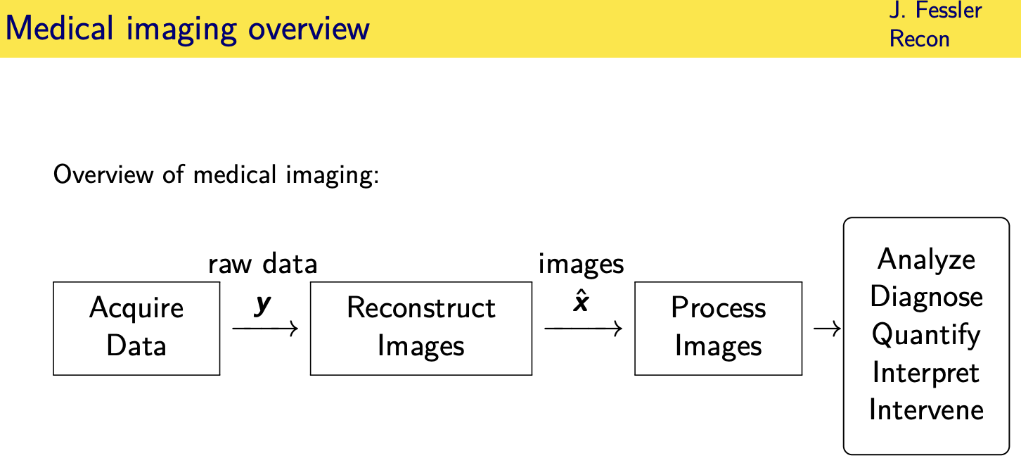
Measurement model
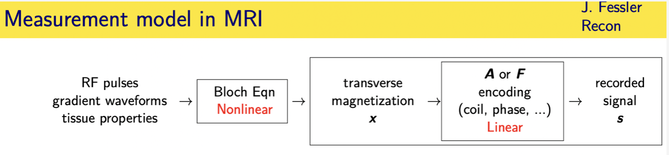
in mri we have enormous can we as engineers have enormous control over the inputs to the system
1.------->we design rf pulses and gradient waveforms that are played if you will into the patient who has their own tissue properties
and then the magnetization the object evolves according to an
2.------->ordinary differential equation called the block equation that's non-linear
3.------->that leads to induced state of transverse magnetization the object
4.------->and then we we sense that transverse magnetization using the gradient waveform properties an encoding matrix that sometimes will be a and sometimes f in this talk
5.------->and that's a linear model between the transverse magnetization and the recorded signal

and so i will be focusing mainly on this part of the the model here going from
the recorded signals back to an image of the transverse magnetization quantitative mri
deals with the topic of going from that
further back to quantifying the tissue properties
and like i said that's a whole other talk all right
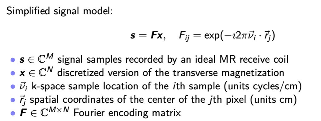
we'll have samples basically in a simplified model of the fourier transform of the transverse magnetization
----->and our goal is to reconstruct that unknown transverse magnetization from those samples
all right so this is the notation i will be using
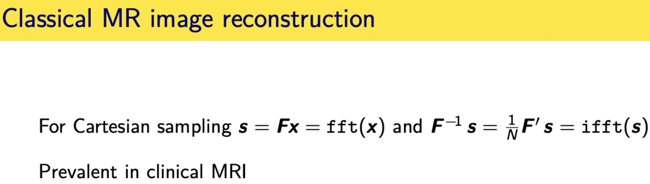
and i'd say probably more than 90 of clinical mri scans fully sample the 2d fourier space on a
cartesian grid
---->so your model is basically that the recorded samples are an fft
of the discretized version of the transverse magnetization
---->so you simply apply an inverse fft to the recorded samples and that gives you the image
and that's what's used primarily in clinical mri even today
so that's that would be the end of the talk if that's all we did because that
would be the reconstruction algorithm right there one called ifft
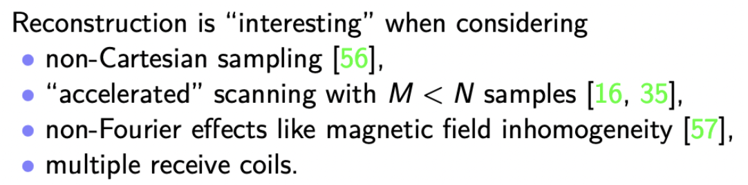
we're going to focus on the more interesting problems and it becomes interesting in three or four different situations
1.(CS)---->one is when you have non-cartesian sampling and others when you collect fewer samples than the other number of unknowns in the object so you have an underdetermined problem that's the
compressed sensing framework
or and i could describe this as a simplified model in reality in some kinds of scans you have to deal with other effects that don't fit into the foray framework
such as magnetic field and homogeneity or in combination with the others
if you have multiple receive coils because this this formula here is for a single received coil
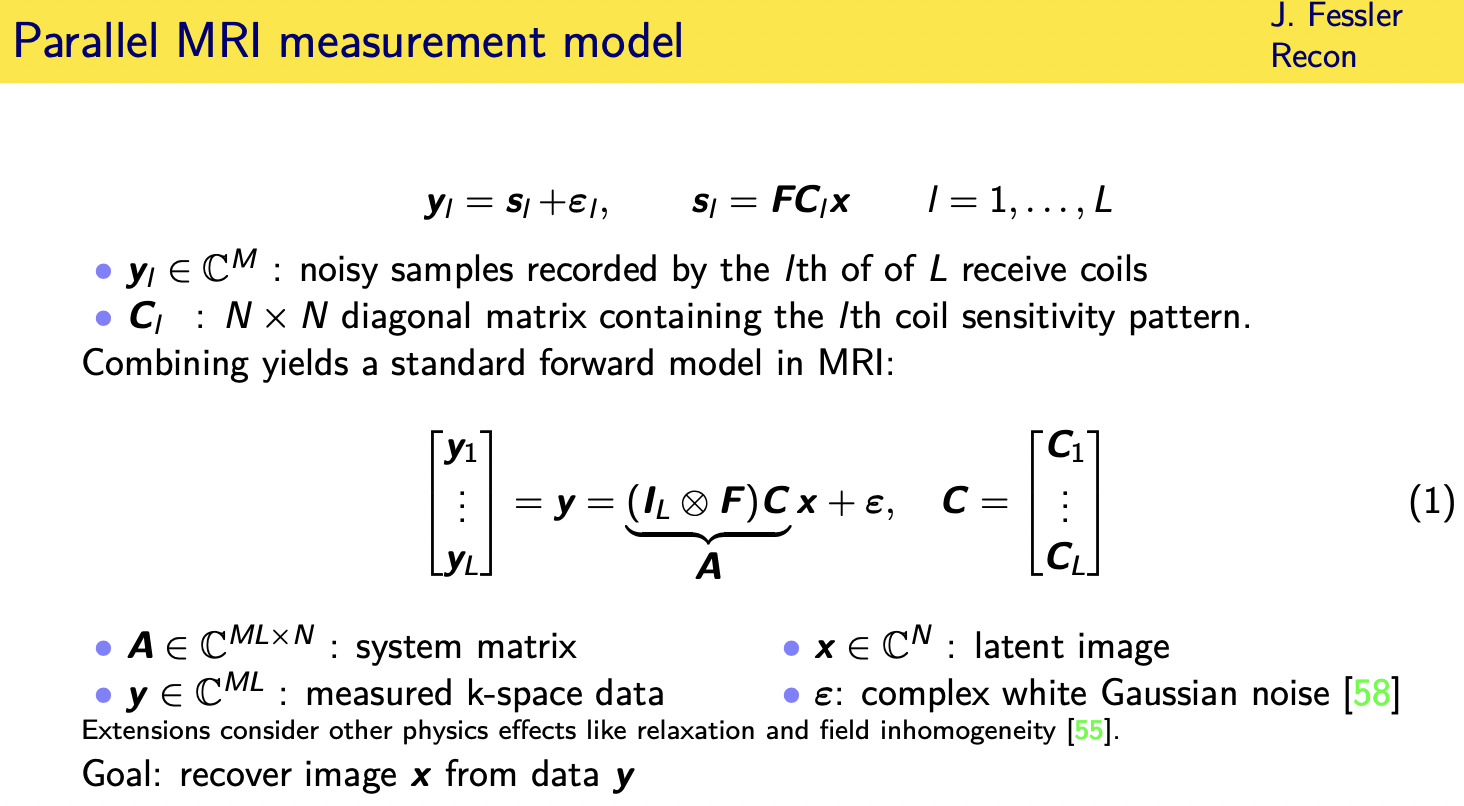
--->so let's move on to the case where we have multiple received coils and now
let's actually acknowledge the fact there's also noise in the data
so let's assume we have l received coils
----->so the samples recorded by the elf coil are an underlying magnetization pattern as seen
through the wrist the coil sensitivity of the alter C of coil
---->and then we have our fourier encoding and then plus noise so this c sub l here is a diagonal matrix that has the coil sensitivity patterns along the diagonal

and i you know coil that's on the right side of the head is more sensitive to
the spins coming from that side of the head than a coil that's on the other side pad
so if we take the measurements from all l coils and stack them up into tall vector
then we can write that you know using a combination of a chronicler product here
and stacking up the coil sensitivity matrices
---->and finally end up with a model of the form y equals ax plus noise and this may be over or under determined depending on how many coils
you have and how many samples in k space that i'm assuming you're collecting m samples in k space
and by the way it's the exact same no matter how many coils you have it's the exact same
samples in k space for each coil so
that's the why there's a chronic product here because each coil seems to sees the same fourier encoding
all right this is still a simplified model like i said there's more some situations need to consider things like relaxation field homogeneity
but i'll just focus on this model in this talk
and of course our goal then and any inverse problem is to recover x from the measurements y
brief review of classic methods
Ordinary least-squares reconstruction
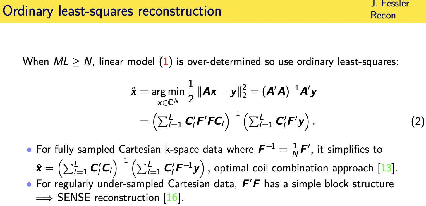
if the product of the number of coils times the number of case-based samples per coil is bigger than the number of pixels
then this is an overturned problem and so you could try to use ordinary least squares
all right which of course has the standard pseudo-inverse solution
you plug in the particular form for the fourier encoding and the coil matrices
and so on and you get this form
we can write this down on paper but in general this is not practical to implement
because this matrix here would be too large to store and invert this matrix here would be n by n
where n is the number of pixels and even in 2d imaging you might have a 128 by 128 image
so this matrix would be 128 squared by 128 squared
now if you fully sample k space then this inner matrix here f transpose f is just a constant times the identity and then it does simplify to just being the inverse of the sum of diagonal matrices which is trivial and this is called the optimal coil combination approach you're basically taking
each the data from each coil taking the inverse fourier transform of that
and then doing a kind of a weighted combination of those based on the coil sensitivity patterns
there are some other under sampling patterns
where f transpose f has a certain simple block structure that you can solve non-iterably that's known as classical sense reconstruction
we're going to be focusing on the case
where the sampling pattern is irregular and there's no such simplification
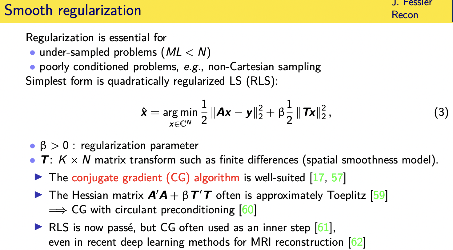
Smooth regularization
non-cartesian && regularization
and in fact in general for general sampling patterns including non-cartesian sampling
that problem is ill-conditioned and so we have to include some form of regularization
and sort of the simplest form of regularization is a quadratic regularizer
so now we're finding reconstructing the image by reconstructing a cost function consisting of two terms
---->one term that measures how closely do we agree with the data
all right or how much do we not agree with the data it's kind of a misfit to the data
---->and then another term that in a bayesian setting would be a log prior
negative log prior that that encourages images to concur with our prior expectations of what images look like
so if we expect images to be smooth
for example we could make this matrix t to be a finite different matrix that looks at the differences between neighboring pixels
if we don't put such a regularizer, there then we will just be fitting the data, the data has noise and we get a very noisy images very irregular
this term can encourage neighboring pixels to be similar and we will avoid having so much noise
all right so this already is a non-trivial optimization problem
it's quadratic so i guess in setting the field of optimization
it's not too hard and conjugate and gradient algorithm
is well suited but there is an
analytical solution here but the
analytical solution depends on this inverse the hessian matrix that is impractical to compute in practice
so we use typically conjugate and gradient algorithms sometimes with a circular pre-conditioner


now i realize some of you are sitting there thinking wow this is really old school why is he talking about this this is 20 plus years old
the reason i'm mentioning it is that many modern iterative algorithms including deep learning algorithms actually have a conjugate gradient step as an inner step of those algorithms
so i think it's important to have that background before we get into the more advanced methods
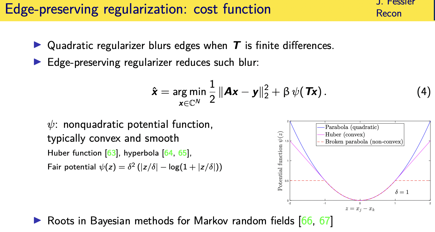
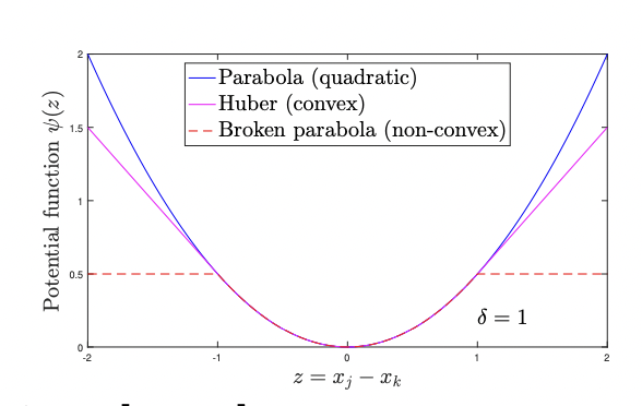
now many of you i'm sure aware that using a quadratic irregularizer hasnthe effect of blurring edges because it strongly penalizes the difference between neighboring pixels a parabola as it rises rapidly really discourages the difference between neighboring pixels
so often we would replace that quadratic function with a non-quadratic function often convex and smooth such as the huber functions shown in magenta here
and since that uber function rises less rapidly than quadratic it penalizes less the difference between neighboring pixels
and so it better preserves edges in the reconstructed image compared to using a parallel or a squared function there
one of my personal favorites of this is the fair potential
as a particularly convenient form when you take its derivative and these kinds of methods also have their their roots invasion methods for markov random fields where these are the energy the potential function
language even uh has its roots as related to energy functions in markov random fields
this is now a non-quadratic cost function
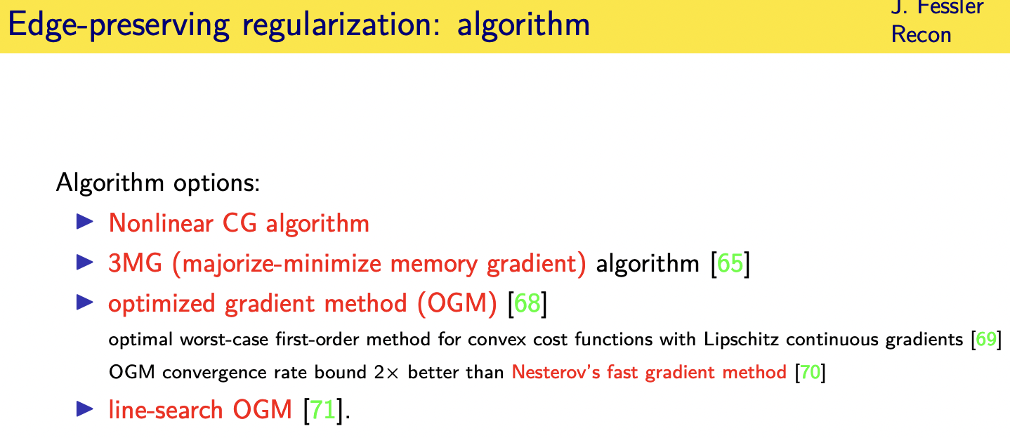
and so you need a different
optimization algorithm for it
and there's a variety of algorithms that
use a non-linear conjugating algorithm
that's particularly effective
one of my former students developed
something called the optimize gradient
method that is
uh improvement on the famous nesteros
fast gradient method that has the worst
case
first order convergence uh of all for
all convex functions with lipschitz continuous gradients
and recently uh group has come up with a
line search
generalization of that optimized
gradient method
so if you have an arbitrary cost
function like convex cost function like
you might have in machine learning
that's smooth
lipstick's continuous gradient this
optimized gradient method
might be a good way to my good good
technique to use it turns out mri the
cost function is almost quadratic
even if you use a fair potential with a
with a nearly
a pretty small value of delta so think
of this as like l1 almost but with a
corner rounded maybe i should have made
that point back in this picture if you
take this magenta curve here
and make delta small enough it's almost
like l1 but the
it's differentiable because you can round at the bottom of the absolute value function

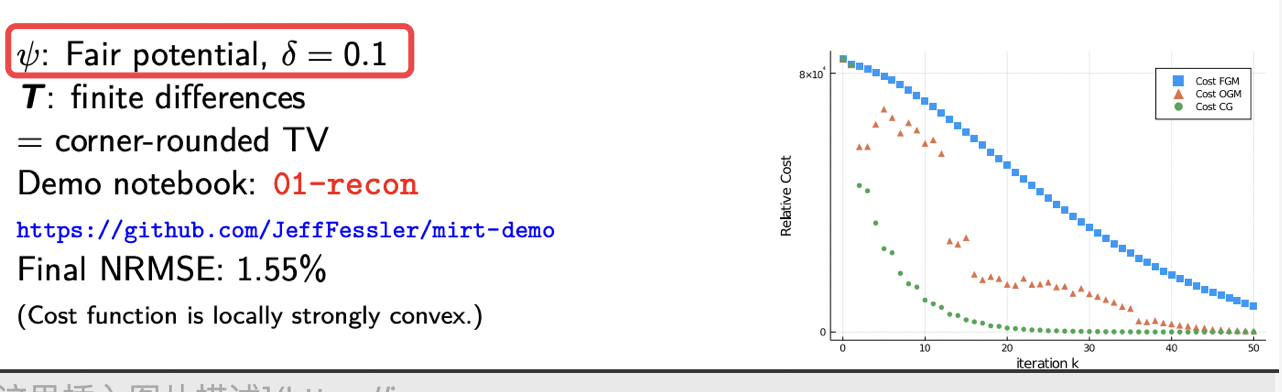
so here's the first concrete example that is one of
the ones you could reproduce yourself
using the demo if you want where i've under-sampled k-space in this pattern so 0
0 the center of k-space the dc the low frequencies are here and so we're fully sampling the low frequencies and then under-sampling these other frequencies with a total of acceleration i think of a factor of four
so i think there's only a fourth of the overall samples are being recorded here this is the true shep logan phantom in the simulation if you just take this data and then do an inverse fourier
transform of it and look at you get this image that i hope you can see over zoom has all sorts of ringing artifact and aliasing artifacts in it the ringing kind of comes from the
if you will the truncation of k space here and the little ripples and so on come from the random sampling outside so this would not be an acceptable image
but if you take this same data and you put it through the cost function i showed on the previous slide and minimize it with some algorithms you can get this edge preserved reconstruction
you can see has pretty close agreement to the ground truth
and by the way there's no sparsity here
no explicit sparsity right it's just
edge preserving regularization
i compared three different algorithms
here as a function of iteration plotting
the cost function and so
the blue curve here is nestoro's famous
fast gradient method or accelerated
gradient method it's sometimes called
the orange triangles here are this
optimized gradient method that has a
worst case convergence bound that is a
factor of two better than
than nesteroff's algorithm and you can
see that you know you you reach any
given point on this
about about in half as many iterations
but for this particular cost function
even though it's non-quadratic the
nonlinear conjugate gradient algorithm
converges even faster and i think the
reason for that here is
this cost function is probably locally
strongly convex and ogm and fgm are not
optimal
for functions that are locally strongly convex whereas cg is quite effective in that regime
and the final root mean squared here is only 1.5 percent so that's quite good
despite the factor of you know
four-fold acceleration k-space so this is motivated of course tons of research on sparsity kinds of models and compressed sensing
Sparsity regularizers:Basic
sparsity models:synthesis form
compressed sensing led to quite a few different optimization algorithms
many of those optimization algorithms have served as the foundation for deep learning based methods
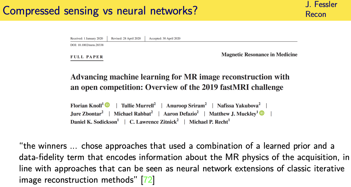
where the current research is so in fact there was just uh recently a paper uh describing a
challenge for mri reconstruction where several groups submitted to a leader board
advanced machine learning based methods for reconstructing knee images from training data
and all three of the winning groups
you this is a quote from the paper chose
approaches that used a combination of a learned prior so that's the machine learning part
and a data fidelity term that encodes information about the mri physics of the acquisition
in line with approaches that can be seen as neural network extensions of the classical iterative inner image reconstruction methods
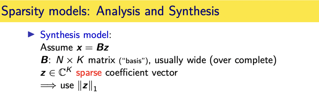
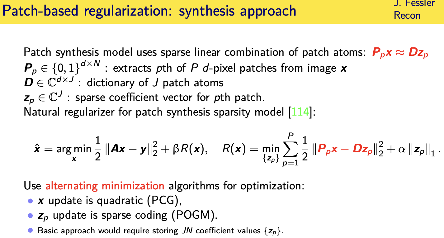
sparsity models:analysis models and synthesis models
so in this field of sparsity there's
sort of two main categories of sparsity models
analysis models and synthesis models so
in a synthesis model
you assume that your unknown image in this case can be synthesized as a linear combination of some columns of some matrix using a sparse set of coefficients and i use the letter b because you kind of think basis but you don't say basis
because usually this matrix is wide so it's over complete
so it's not it can't be can't have
linearly independent columns so strictly
speaking can't be a basis but
in a in a sense it's like a basis all
right and
since you expect in this model and again
you know there's this expression that i wrote the bottom of the page all models are wrong
some models are useful it's very debatable whether any real world images and mri actually satisfy this model exactly

but if you're going to under sample case-based data you have to impose some kind of model to make up for the missing data and
the models on this page are two of the models that have been used effectively
uh to make up to sort of reduce the degrees of freedom somehow in the reconstruction problem

so this is one way of sort of reducing the degree of freedom is assuming that your image can be expressed as linear combinations using sparse coefficients
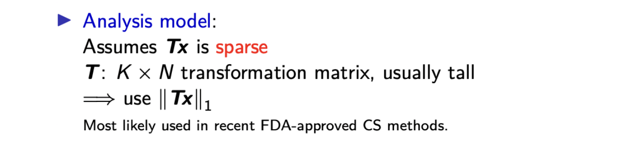
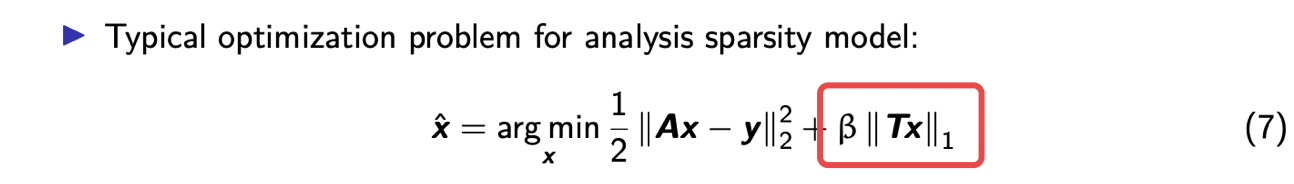
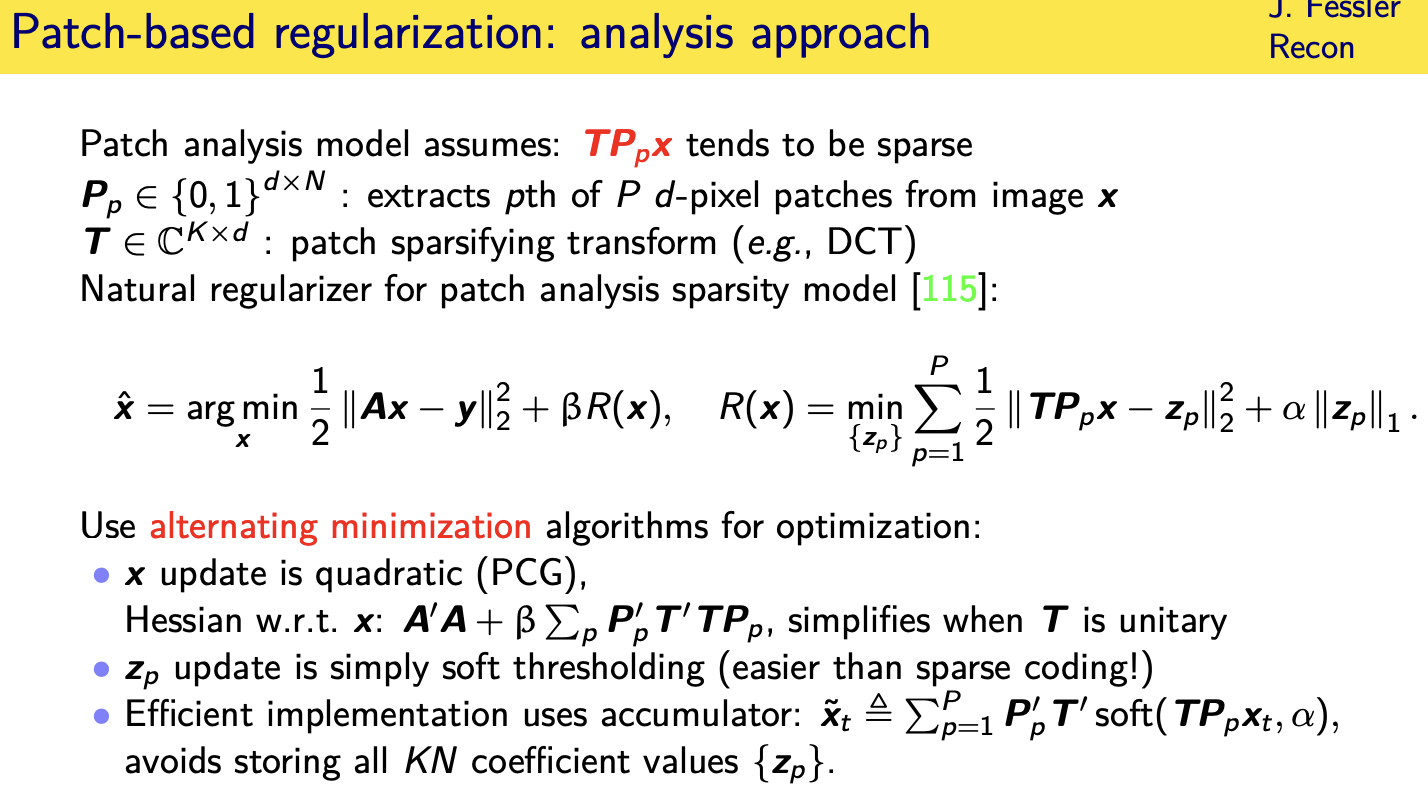
so the dual this is an analysis model
where you assume you have some matrix t
a transform matrix you apply to your
image and the result of that matrix vector product is a sparse vector so in that case you
might use a regularizer that involves something like the one norm of the product t times x because you're assuming that
that that product is a sparse vector
at the time i first made these slides i
said this was most likely used in the
recent fda approved compressed sensing
methods i've since had conversations
with people in the companies and i know
a little bit more about what's under the
hood and this is indeed
the kind of regularizer that's being
used as we speak
in the compressed sensing methods at least in some of the companies compress sensing products
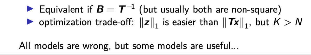
these two models turn out
to be equivalent if the matrices are square and
one is in the invertible and one is the inverse of the other
but usually they're not square usually the
basis excuse me the dictionary we use
here is y
so over complete and usually the
transforms are tall
all right and i'd say this is still
somewhat
a debate in the field of which of these models is preferable
um using this model is a little bit
easier because your one norm is applied
directly to the coefficients and there's
no matrix inside of the one norm so it's
a little easier for the computation algorithms
on the uh whereas with the analysis
model you have a matrix inside the one
norm that makes a little bit harder for optimization

but on the other hand you'll see in a second that the synthesis model usually has more unknowns to manipulate because the number of coefficients here is usually bigger than that n and so that's there's a potential trade-off there
proximal optimized gradient method
so let's dig into that a little bit more
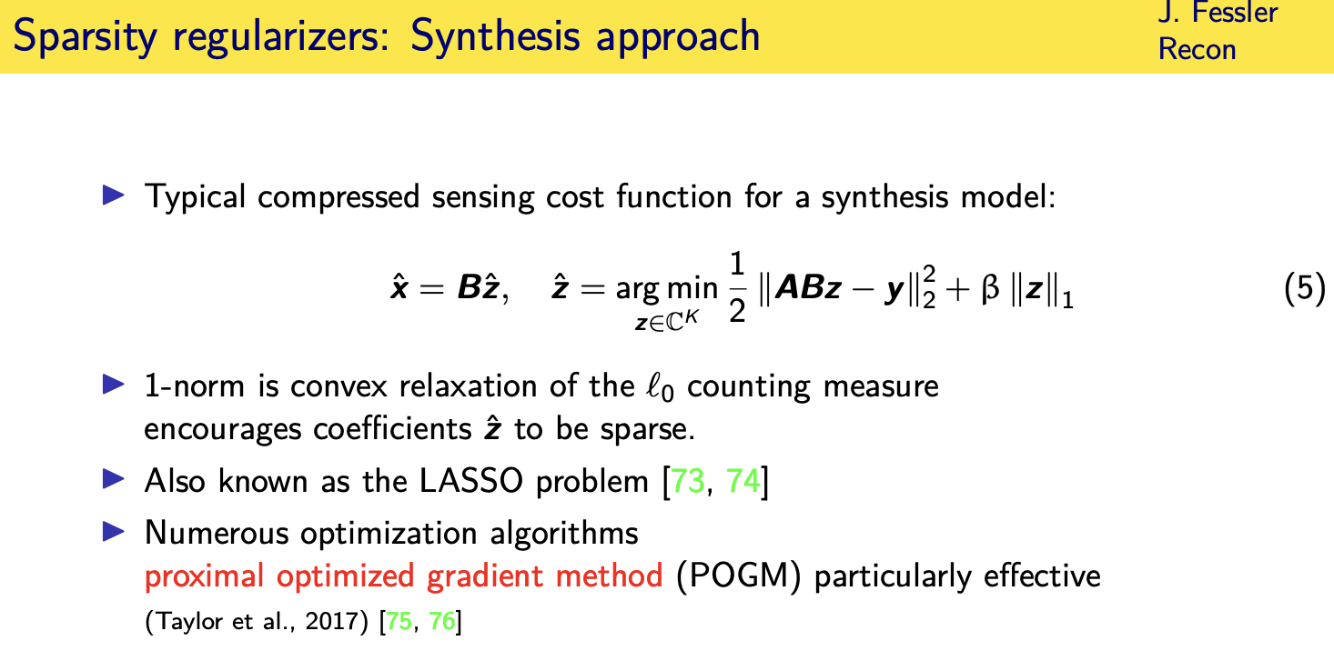
so if you believe in the synthesis model
if you believe your image can be
represented as a linear combination of
some
columns of a dictionary then this is a
logical way to set up the optimization problem
find the set of coefficients that when i synthesize an image from those coefficients and then propagate that to k space i get agreement with the data
but at the same time i want those coefficients to be sparse
all right so this is a convex optimization problem
it's convex because we use the one norm
instead of a zero norm here to count the
number of non-zero coefficients and
uh and there's a famous problem in
statistics called the lasso problem and
there's lots and lots of optimization
algorithms for it many of you have
probably used
if you've worked on a problem like this
you've probably used ista the iterative
soft thresholding algorithm or you might have used
fista the fast iterative thresholding algorithm i'd like to encourage you to
look at an algorithm called the proximal optimized gradient method
that is an improvement on fista and i'm going to show results
Proximal methods
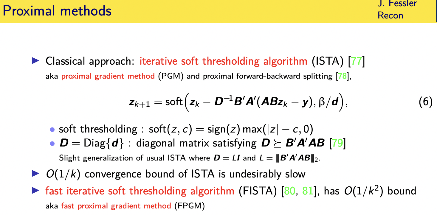
iterative soft thresholding algorithm
the iterative soft thresholding algorithm also known as the proximal gradient method basically takes a descent in the gradient direction so this is the
this right here is the gradient of that cost of this data fit term
in the cost function i just showed you
and then it applies soft thresholding
to that gradient update and because soft
thresholding is the proximal operator
associated with the one one all right so
very simple algorithm

uh the classical version you'd have a step size here i actually tend to use a different version that has a diagonal matrix here that satisfies a certain
majorization condition
and the reason i you i do that is that
the classical um approach
requires finding a lipschitz constant
which is a spectral norm
that is often inconvenient to compute
these matrices are really large and so
computing
spectral norm can be quite quite
expensive
whereas i have uh references here on
tools for finding an
easy to invert you know diagonal matrix
that satisfies this
inequality meaning d minus this product
is a positive semi-definite matrix
and that doesn't require computing any
spectral norms
so that's the version that i tend to use
unfortunately this algorithm as simple
as this has an order one over k where k
is the number of iterations convergence
rate which is annoyingly slow and that's
why people tend to use fifth instead
because it has an order one over k
squared bound which is a huge
improvement this is also known as the
fast proximal gradient method
a drawback in my view of the synthesis form is that your final image is going to be
in the span of your matrix b so you have to really believe that you have a reasonable basis
now excuse me over complete dictionary that a linear combination of those columns can represent the image that you want
this is not an approximation this is an equality this is saying i'm going to finally
synthesize my image using my basis
excuse me using my dictionary and you
know that's an
open question whether we really know the
right models to use in imaging so that's
a drawback i think of that form
potential drawback of that formulation
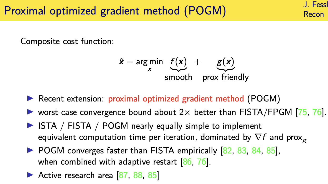
composite cost functions
this is a sum of a
smooth term
plus a non-smooth term all right and
such cost functions are called composite cost functions when you have a sum of a
smooth term typically a data fit term
and then some non-smooth term typically
a regularizer often involving sparsity or constraints
and typically when people focus on composite functions
composite cost functions they're
considering non-smooth terms that are
what are called prox friendly it's easy
to compute the proximal operator for
those
and my favorite algorithm these days for
this kind of cost functions called the
proximal optimized gradient method
because it has a worst case convergence bound that's about two times better than fista
and in practice my observed case
performance is
similar to that factor of two
improvement that the worst case theory
tells you and i'm going to show you the
code in segments extremely
simple to implement if you've
implemented fista it's like a one-line
change to make it fpgm
same amount of time per iteration most
of the time is involved computing the
gradient of the smooth term and then
depends on your how friend prox friendly
your proximal term is
but i want to point out even though
that's my current favorite this is an
active research area and there's there's
people continuing to push on making a
faster algorithms for this particular
family of cost functions
first of all
if you have more than two smooth
functions you would just add them
together and that would still be smooth
i bet that's not what you meant
i bet you're wondering if your prox term
has
more than uh one non-smooth function so
you might have for example a one norm
and maybe a constraint in ct you might
have a non-negativity constraint
now that particular combination i just
mentioned there
um a one norm and that still can be
combined into a single
non-smooth term that is prox friendly
but if you had something like
you wanted total variation plus a
non-negativity constraint
well tv by itself is already not prox
friendly
and then if you add other things to it
it's even less friendly i think
and so i think my answer to question is
i'm not i mean
i don't know of any general case uh way
to handle more than two
prox friendly terms there is a field
i'll just mention a term there's a field
called
there's a a method called proximal averaging
where if you have multiple non-smooth
terms each update
uses just one of those terms and you
sort of cycle through the different
terms or you
or you apply them individually and then
you take the average and the
average of a set of proximal functions
proximal operators is
in general not the same as the proximal operator of the sum of those functions but people
have made inroads into some convergence
theory even though you're sort of
applying those non-smooth terms one
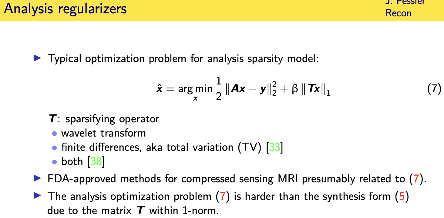
in an analysis model you don't
you don't have that kind of same hard
constraint you put an analysis
regularizer in you still have your data
fit term as it is you're finding an
image that trades off
fit to the data and in this case
sparsity of some transform of the image
but you never require that your image
lie in the span of any particular operator
so i feel like this might be a little
bit more robust to um
having an imperfect choice of the
operator here you know and all choices
are imperfect yeah you know
the most common dif uh choices for this
matrix t
are the wavelet transform some wavelet
transform finite differences and if we
use finite differences that's related to
total variation or
in the original sparse mri paper by
mickey lustig at all they used a
combination of both of those
operators which you could think of as
sort of just stacking up different
matrices here making this matrix
t even taller and i'm quite sure that
the fda approved methods that are out
there are basically
at least for some of the manufacturers
are related to this cost function
unfortunately this cost function is
harder to
optimize because of the matrix t inside
of the one norm
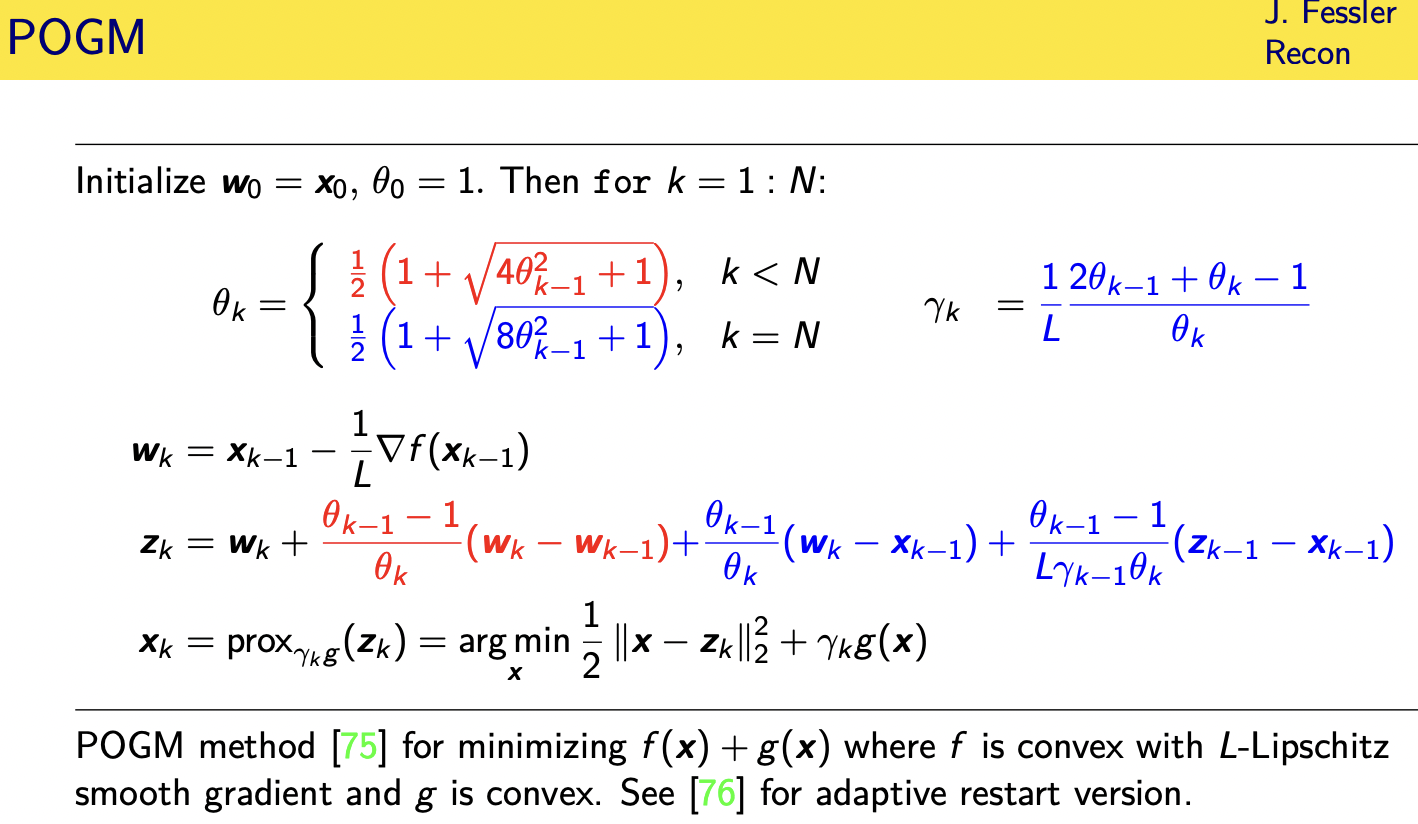
proximal optimized gradient method
this is what the proximal optimized gradient method looks like
so the the parts shown in red here are what you have with fista sophista involves a gradient
step involving the gradient of the data fit term
and then there's these magic momentum
factors that nesteroff somehow came up
with that are kind of mysterious
and then you combine those momentum
factors with a certain update that
involves the difference between these intermediate
uh variables at the previous two
iterations that's the momentum
um and and then finally there and then
at some point in vista there's also a
proximal step which is which in general
i've been saying proximal operator
multiple times and i haven't defined it
here's the definition of the proximal
operator it's the
minimizer of a quadratic term plus
whatever your
function is you're applying the prox to
so if this is the one norm here that
would be uh
the solution to this is soft threshold
so the
proximal optimized gradient method is an
extension of thista if you want that has
these
additional terms that are shown in blue
so there's a slightly different magic
momentum factor for the very last
iteration for the nth iteration
and along the way there's um a couple
extra um
momentum-like terms that involve
differences between
various quantities adrian taylor who
came up with this method
i think uses what's called computer
assisted proof to find this
you can read his paper to learn more
about that
he has nice software tools for helping
develop algorithms in that way
so you can see it's a very small change
to the code it does require maybe
storing one or two extra
copies of variables but that's that's
not a big deal memory wise
uh and you can further speed this up
using something called adaptive restart
so if your momentum
starts to point in direction that is too
different than your gradient
then you often reset and and go back and
and refer to the gradient again sort of
reset if you will to
the iteration counter back to one and
and thereby sort of dampen the momentum
this is especially useful if your cost
function is locally strongly convex
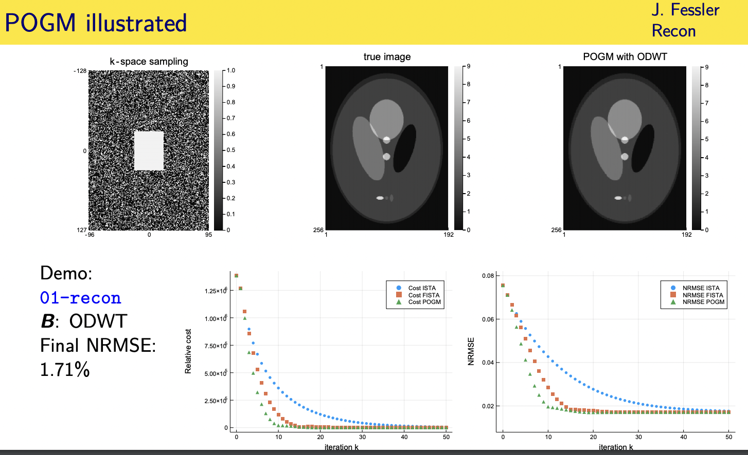
orthogonal discrete wavelet transform
wavelet coefficients
here's concrete example
same data that i showed you before but
now a different cost function i'm using
my b here as an orthogonal discrete wavelet transform
all right and so i have a one norm on
the wavelet coefficients here
and then i'm plotting the cost function versus iteration here and the blue curve
is the classic
iterative soft thresholding algorithm
approximate gradient method
the orange is the order one over skate
over one over k squared convergence rate
you get with fista and then pogm also
has an
order 1 over k squared worst case
convergence rate but with a better
constant and you can see that better
constant leads to
you know additional acceleration it's
not a gigantic additional acceleration
but given that it hardly takes any more
work to implement
in my experience it's worth it and we've
used it for quite a
few different applications
in an analysis model you don't
you don't have that kind of same hard
constraint you put an analysis
regularizer in you still have your data
fit term as it is you're finding an
image that trades off
fit to the data and in this case
sparsity of some transform of the image
but you never require that your image
lie in the span of any particular
operator
so i feel like this might be a little
bit more robust to um
having an imperfect choice of the
operator here you know and all choices
are imperfect yeah you know
the most common dif uh choices for this
matrix t
are the wavelet transform some wavelet
transform finite differences and if we
use finite differences that's related to
total variation or
in the original sparse mri paper by
mickey lustig at all they used a
combination of both of those
operators which you could think of as
sort of just stacking up different
matrices here making this matrix
t even taller and i'm quite sure that
the fda approved methods that are out
there are basically
at least for some of the manufacturers
are related to this cost function
unfortunately this cost function is
harder to
optimize because of the matrix t inside
of the one norm
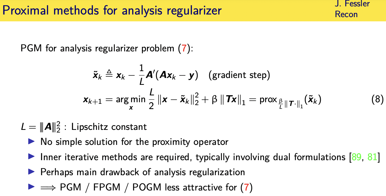
so what are your choices here
you could
try applying ista or the proximal
gradient method you take a gradient step
and then you'd have your proximal
operator step but unfortunately that
proximal operator step requires
minimizing a cost function
it's a little easier than the original
one because there's no matrix in front
of x and the two norm
but we still have a matrix x in front of
the one norm and there's no closed form
solution to that in general unless t
happens to be unitary
so then you need iterative methods to
solve this inner
proximal problem and this is now you
have iterations within iterations and
i'm not
a huge fan if i can avoid it of having
those sort of nested iterations
as i mentioned this is the classical
version where you put the lipsticks
constant here and how easy that is to
compute depends on your application in
single coil mri this is easy in multiple
coil mri it's a little bit harder
especially not in cartesian
parallel mri all right so the
the pogm these kind of first order
methods are not as attractive
for the analysis formulation because of
that matrix t
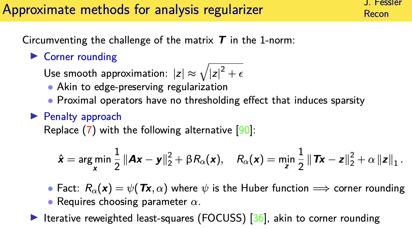
so what can you do well what operations
you can find say well let me just
replace my one norm
with an approximate one norm by rounding
the corner
of the absolute value function lots of
papers have done that and once you do
that you're basically back to edge
preserving regularization and you might
as well use nonlinear conjugate gradient
for it because that works quite
effectively
but then you don't get any pure sparsity
you'll get some shrinkage
of some of the coefficients but you
won't get any zeros once you round the
corner you need that
non-differentiability
there's nice work by mila nikolova to
show that
an alternative approach is you replace
this
excuse me this regularizer right here
with an alternative a penalty approach
that says well
i want an image whose transform
is close to a vector z where i want that
vector z
to be sparse and there's quite a few
papers that use this kind of formulation
so we want an image that fits the data
but we also want to fit
an image whose transform is close to
some sparse coefficients
now it turns out if you do this you can
actually for the one norm here solve
this problem analytically
and it turns out that this just becomes
the same as using a hoover function
so we're back to just a different form
of quarter rounding
and then there's a re iteratively
reweightedly squares uh method that i
won't
talk about more here
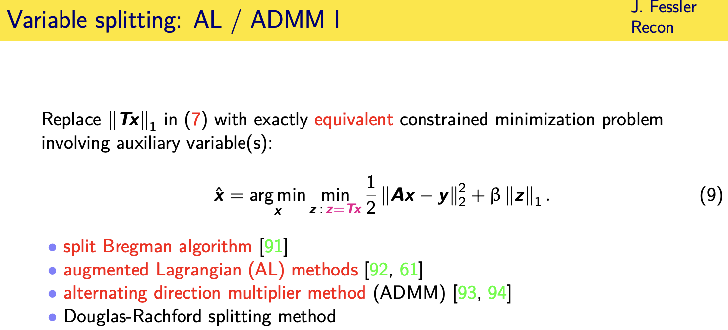
if you really feel like you want the
exact one norm
then probably your best bet is to use an
augmented lagrangian or adm kind of
method where you replace the original
cost function with a constrained version
so you introduce an auxiliary variable z
that you define equal to tx so then you
put that variable z inside the one norm
and now we have a constrained
optimization problem in two variables
we're minimizing over
x and z subject to an equality
constraint
and at least now we've gotten rid of
there's no matrix inside the one
all right and there's a whole bunch of
related algorithms split bregman
augmented lagrangian admm and douglas
rashford
that are kind of all variations of
methods for or
often equivalent methods for solving
this
constrained optimization problem
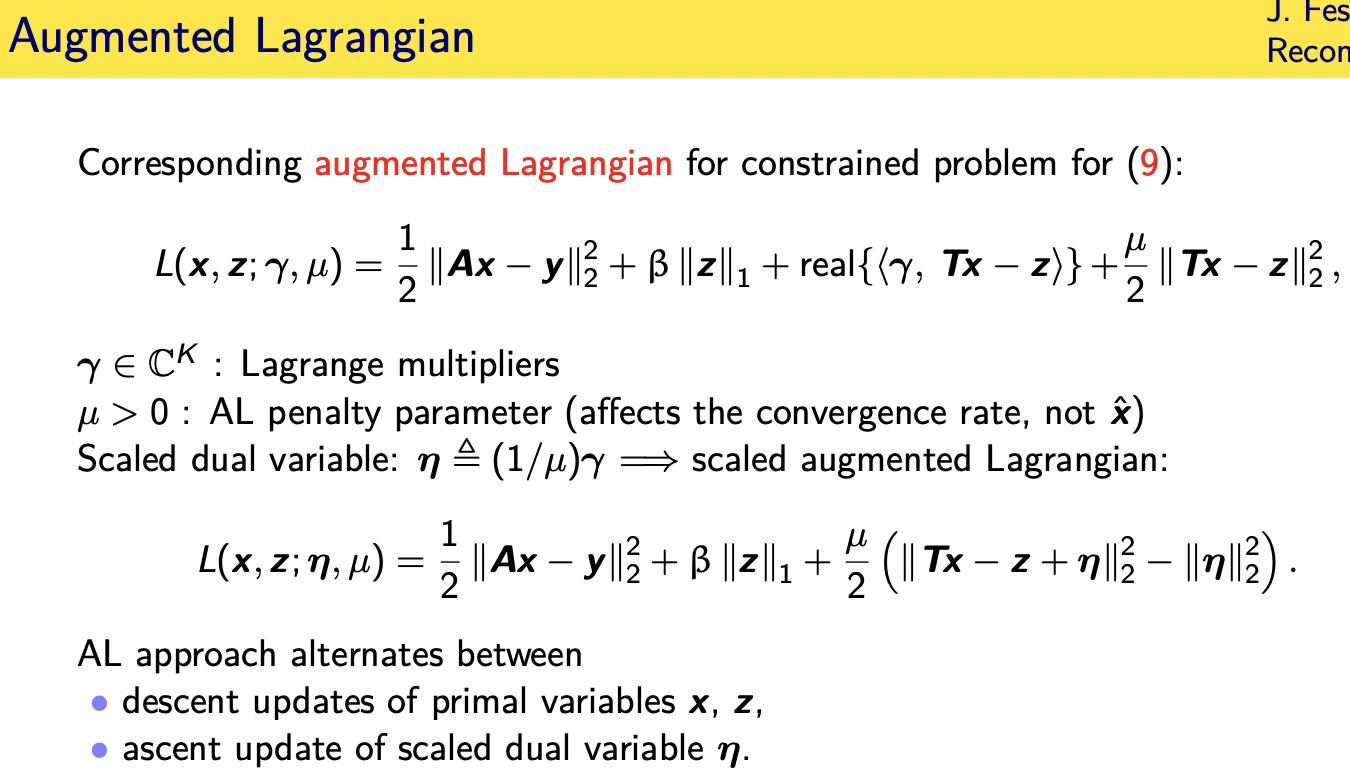
if you write down the augmented
lagrangian for this problem it has your
data fit term has that one norm for the
sparse coefficients
it has a term involving lagrange
multipliers
and then this is the augmented part of
the augmented lagrangian where there's a
quadratic term that
has involves the difference between tx
and z
that came from the initial constraint
that we want in the limit t
x d equals z this parameter zero mu here
is called a
al penalty parameter this affects the
convergence rate but not the final
solution x hat
um it turns out it's convenient to make
a little change of variable and get
something called the scaled augmented
lagrangian which now has these four
terms in it
so there's there's really two primal
variables here x and z
and then a dual variable data and we
alternate
between doing descent in adm you
alternate between doing descent updates
of the x variable the z variable
and then a sense update of the scaled
dual variable eta
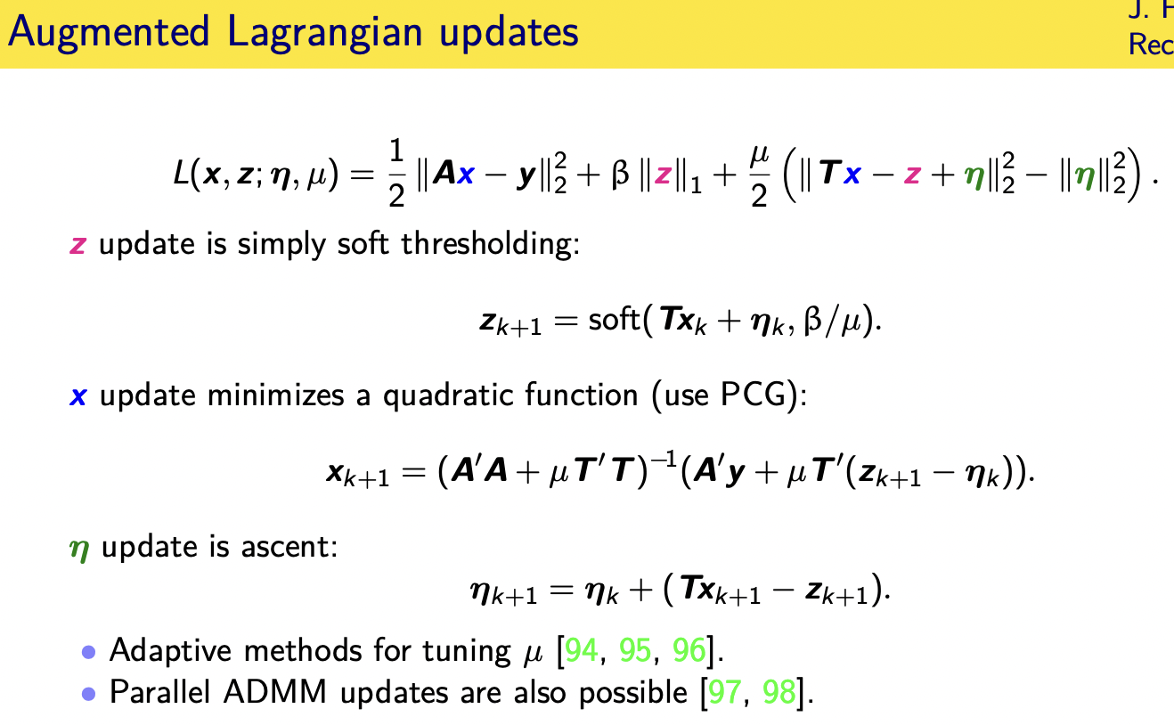
so let's actually walk through that
because again these
versions of this kind of algorithm have
appeared even in the modern
deep learning kind of methods so i've
color coded here things
color coded the variables here so we
have the augmented lagrange in here
there's no closed form solution to this
so we need to apply iterative methods
and we're going to alternate between
these different variables so when we
update
z you notice c just appears in these two
terms here
and this is simply the proximal operator
basically
of the of the one norm applied to the
quantity t x plus eta so we apply soft
thresholding
simple update for z if you look at where
x appears it appears in a quadratic term
here
and another quadratic term here so
that's perfect for using the conjugate
gradient algorithm
so this example of where knowing about
cg for quadratic is really valuable
i've written it here in the closed form
solution involving the matrix inverse
but in practice
uh unless it's single coil cartesian mri
you will probably need to iterate to to
update x and then finally the update for
eta
is in a ascent direction and there are
variations of this for how you choose mu
and other and other variations of this
algorithm so you've taken a hard
optimization problem and sort of
manipulated it to get a sequence of
three different easy updates that you
cycle through
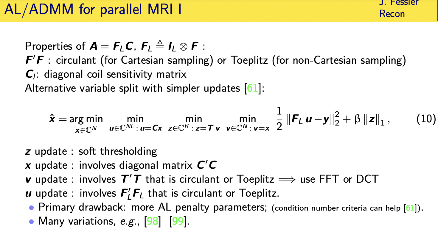
uh turns out for parallel mri there's a
little bit more um
involved but advantageous version of
this where we exploit
what i just showed you on the previous
slide would apply to lots and lots of
applications not just mri
if in the in the application mri we have
some particular structure to our problem
our problem
involves a number under sampled fft and
coil sensitivity matrices
and the under sampled f t has the
property of uh being related to
a fourier transform and f transpose f
has certain properties
the coil matrices are diagonal that's a
certain property
so it turns out it's beneficial to
introduce more auxiliary variables
we'll let u equal cx here we let uh
we still have the sparsity terms equals
tv we let
we introduce z just as an extra variable
with a constraint v equals x
all right and i i don't think i'm going
through all of the details here but just
letting you know that once you make all
of these variables
and then write down the augmented
lagrangian which is much longer now
because we have one two three
constraints plus these two terms so
there'll be a total of
at least five terms involved there um
each of the updates becomes really
simple you don't need any conjugate
ingredient
when you do the x update turns out you
only need to invert a diagonal matrix
the v update involves t transpose t that
is often circulant or toplets so very
easy to invert
the update involves f transpose f that
is circulant in the cartesian case and
topless in the
non-cartesian case so you can really
effectively either just invert it with
ffts
or do a couple iterations of a
of a circular precondition cg but
now there's more parameters to two and
that's the only drawback
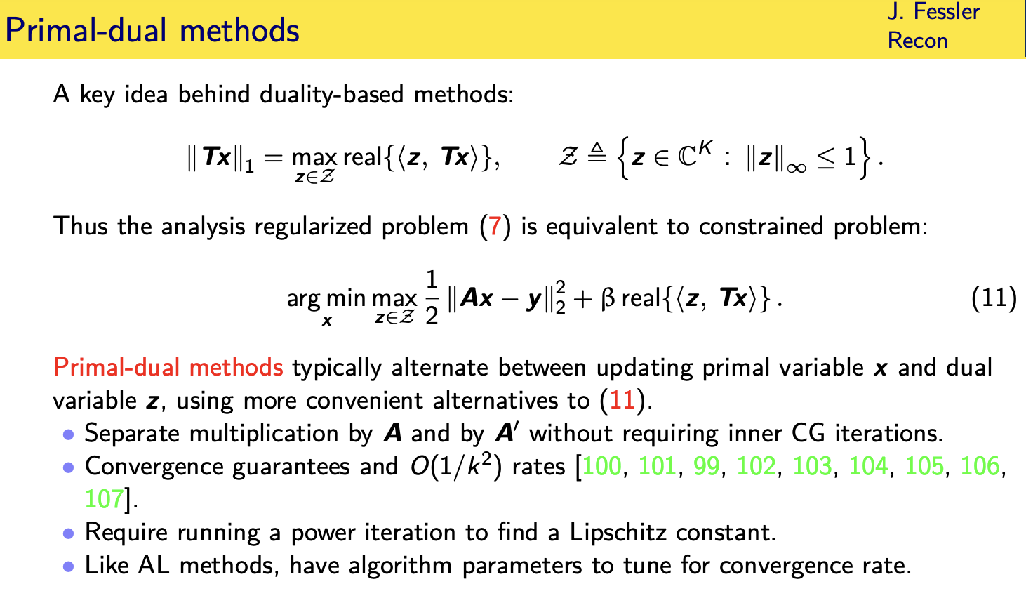
there's also a family of duality methods
for dealing with
this matrix inside than one norm and i'm
not going to give the full story here i
just say the essence of the idea
is that you can rewrite this one norm as
the maximum
over a set of dual variables
whose maximum values of most one of the
inner product of those dual variables
with
t times x so you've
you've replaced in essence the one norm
with an infinity norm an infinity norm
is like a box constraint
and that's kind of easier to deal with
in many optimization algorithms
and so you can rewrite the original
analysis regularized problem
is a minimization over two variables one
unconstrained and one
having these box constraints with
uh now an inner product here and you can
sort of do alternating updates between
x and z i'm oversimplifying but that's
the essence of the idea
so there's a family methods called
shamble pop methods or primal dual
methods relating to
solving it in this form
sparsity regularizers:Advanced
Non- SENSE methods
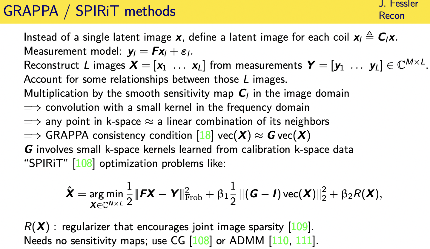
GRAPPA / SPIRiT methods
Calibrationless methods
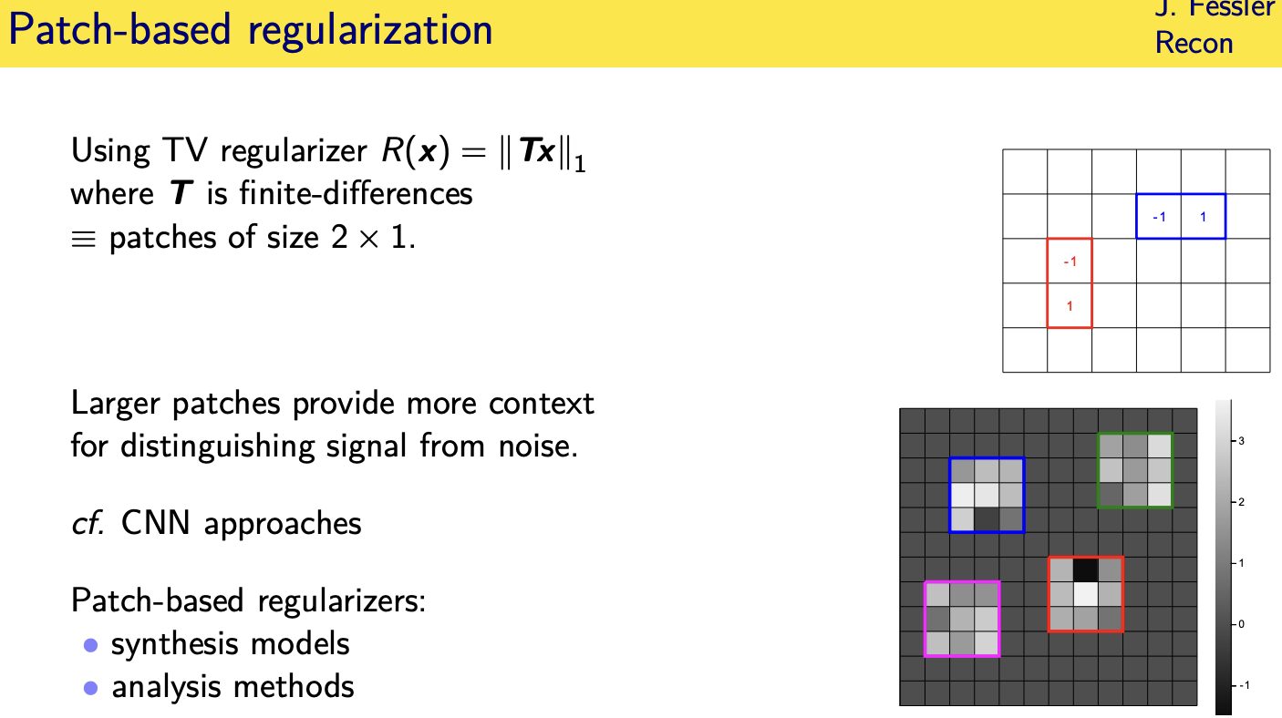
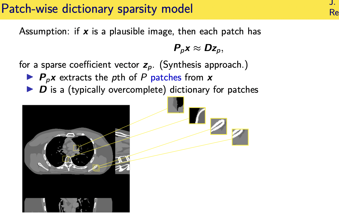
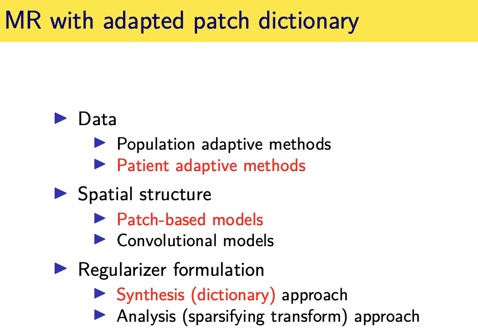
Patch-based sparsity models
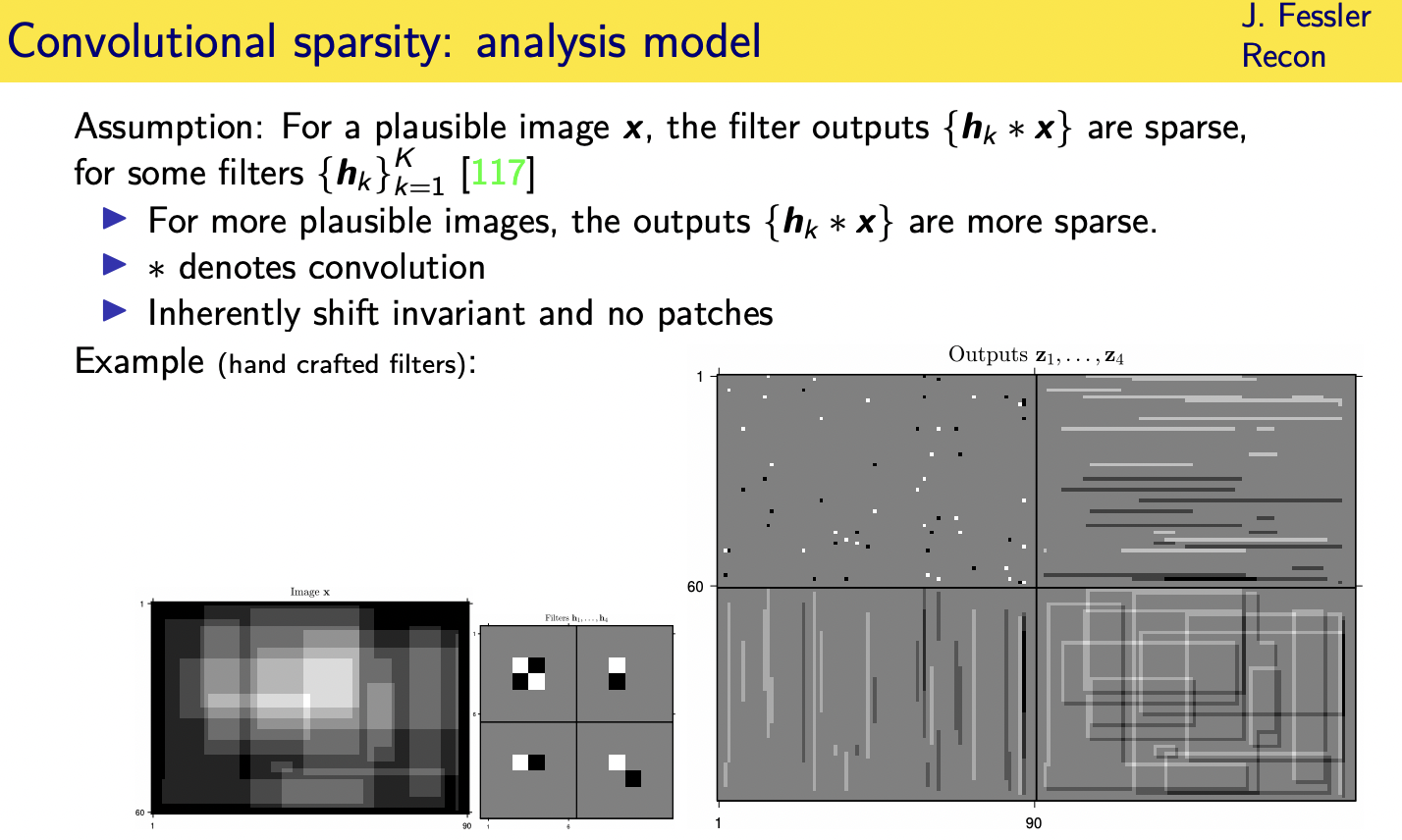
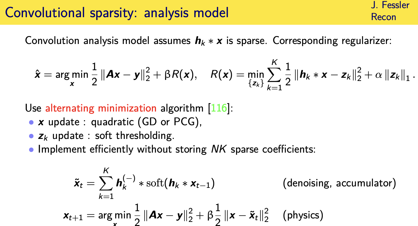
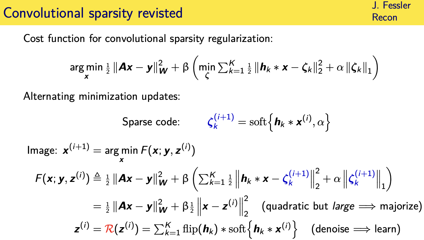
Convolutional regularizers
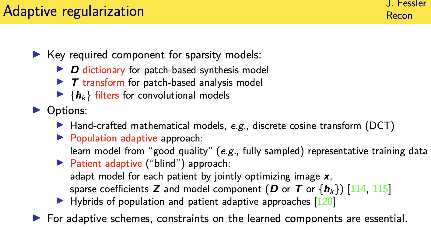
Adaptive regularizers

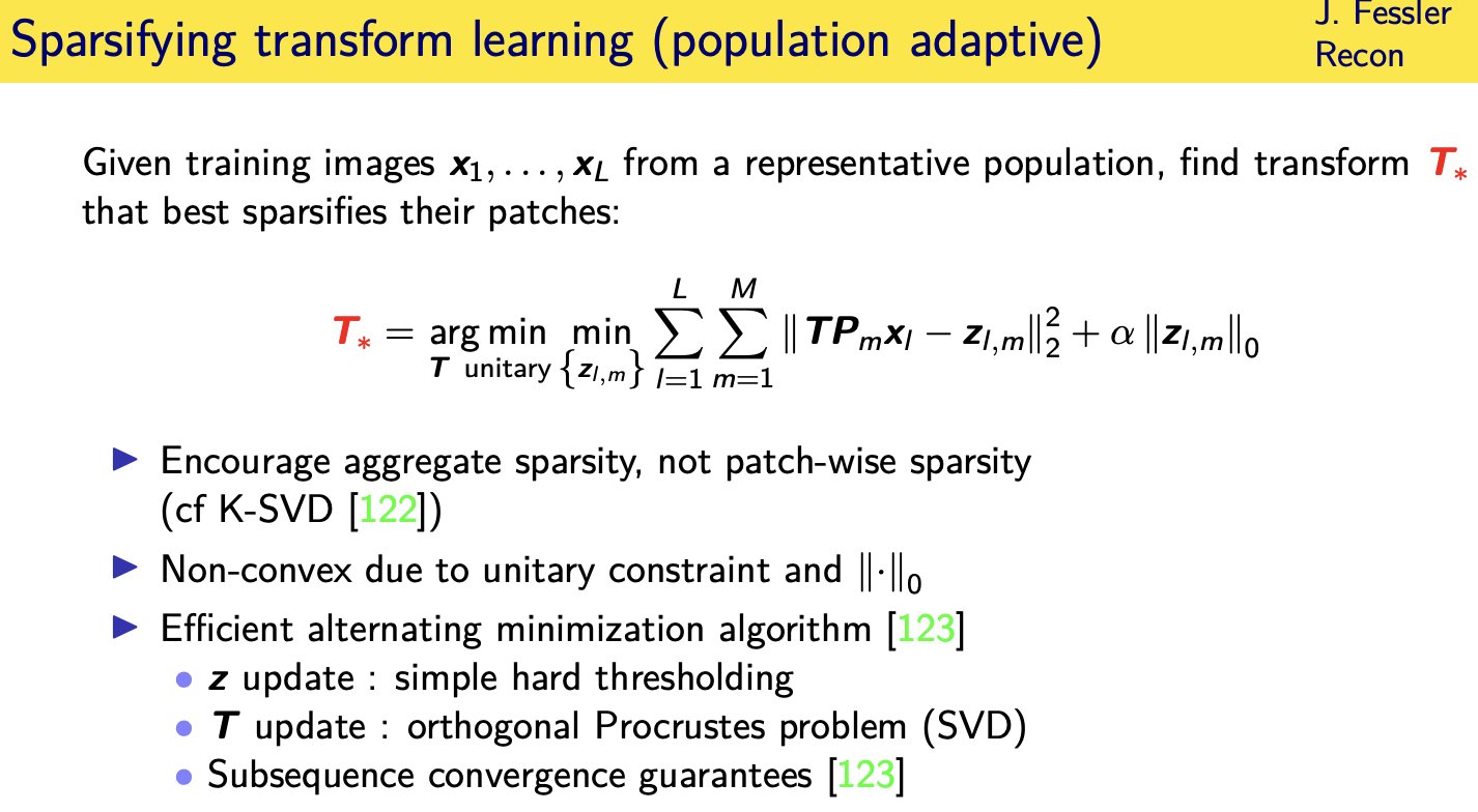
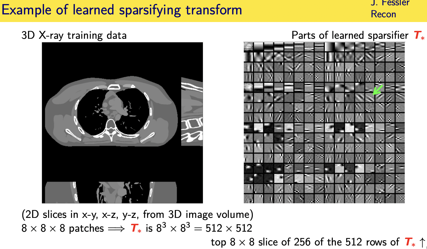
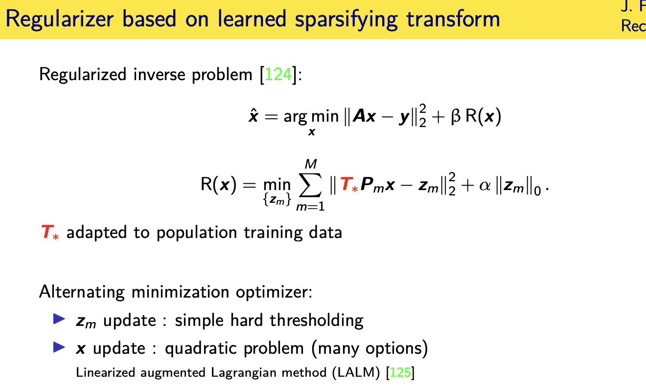
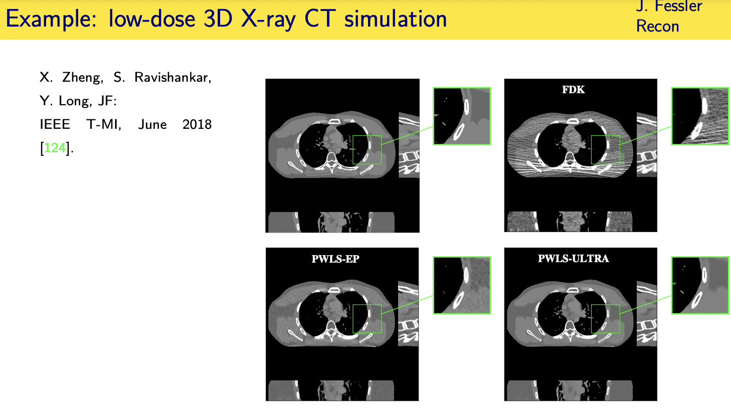
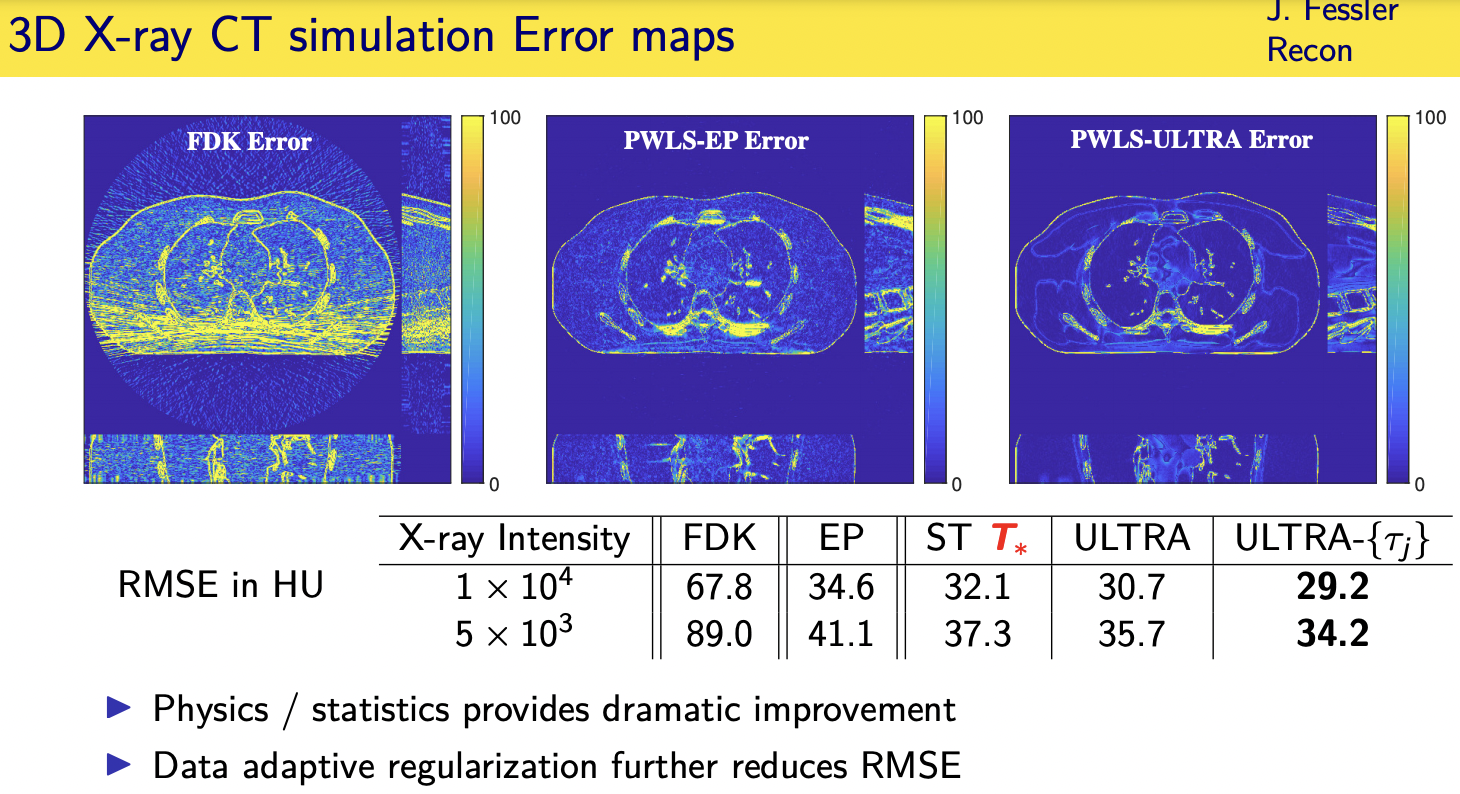
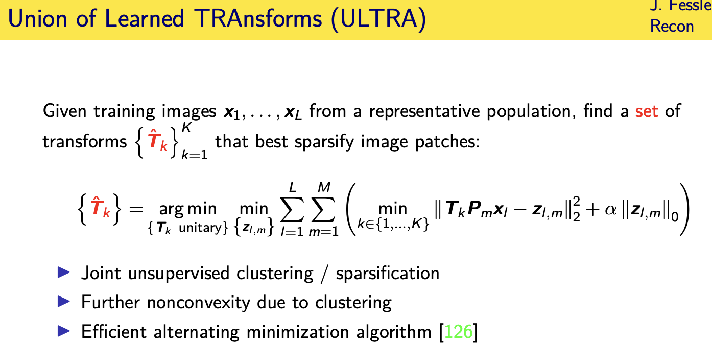
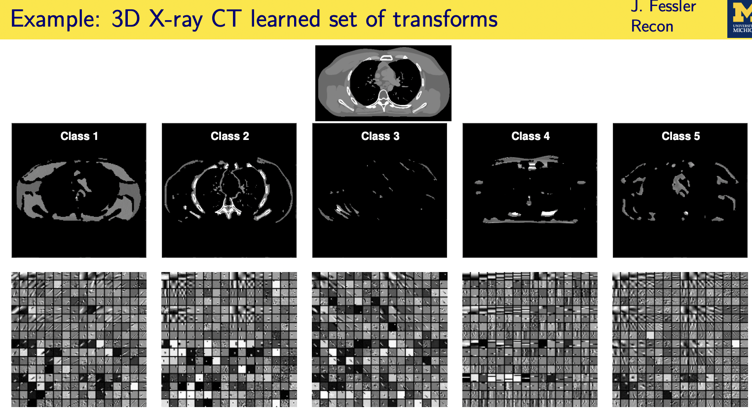
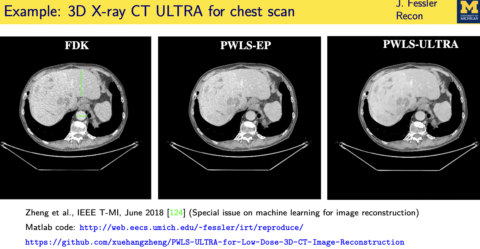
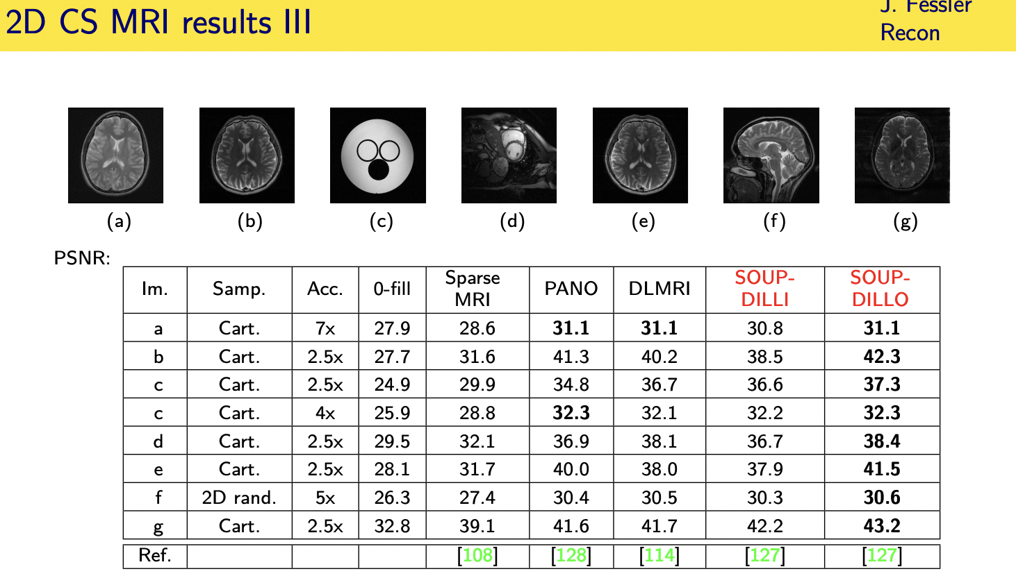
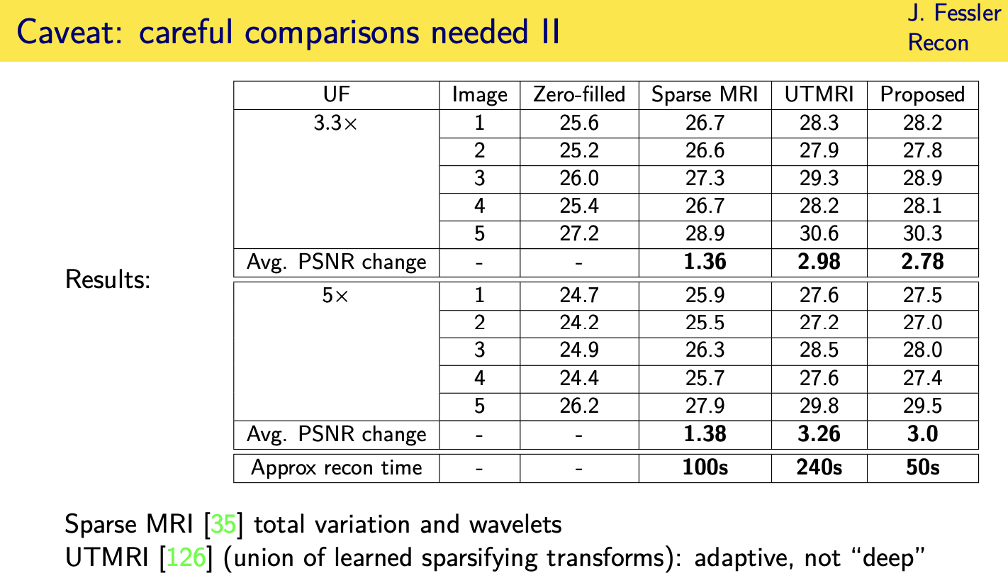
population adaptive regularization---- example:learned transforms
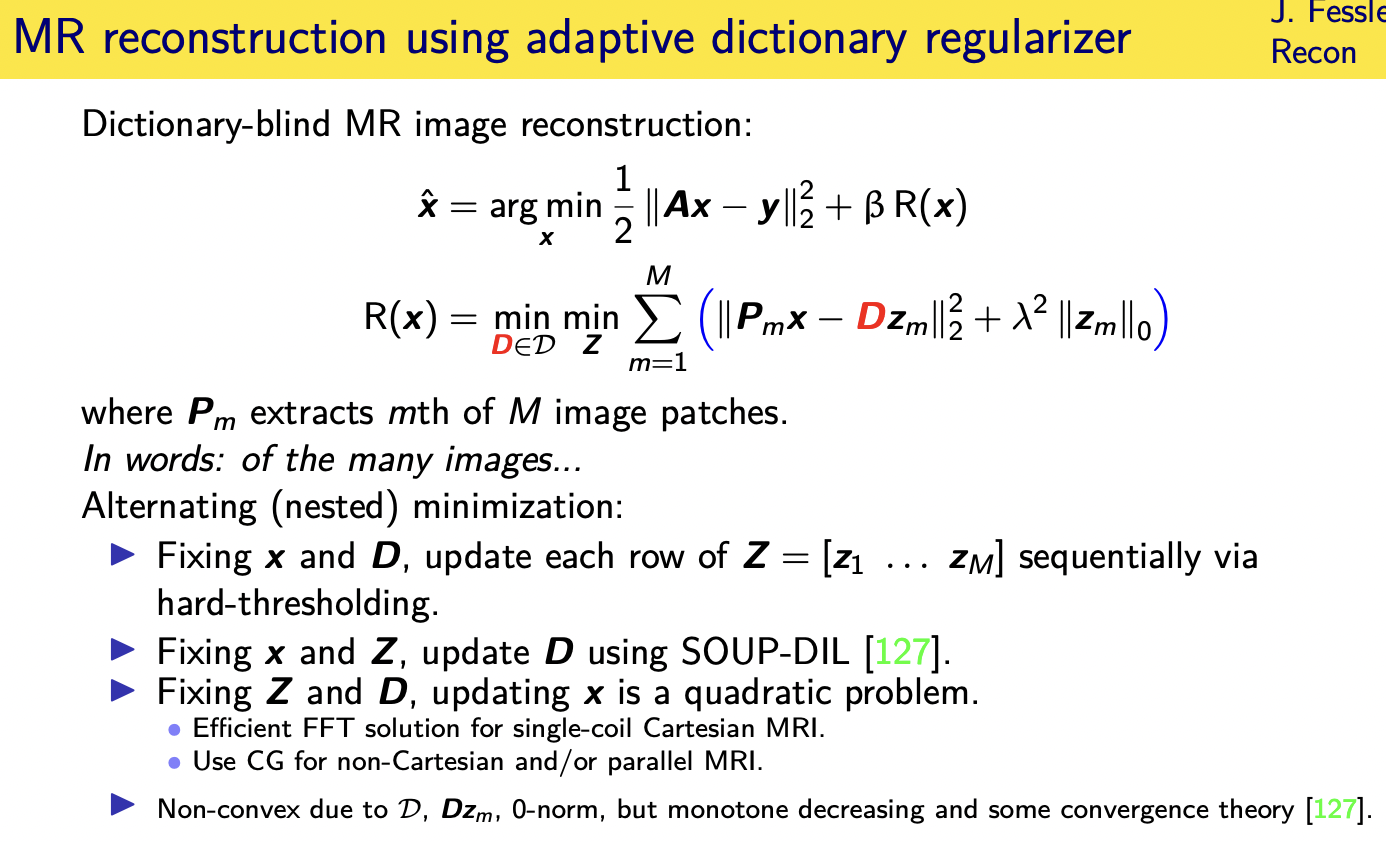
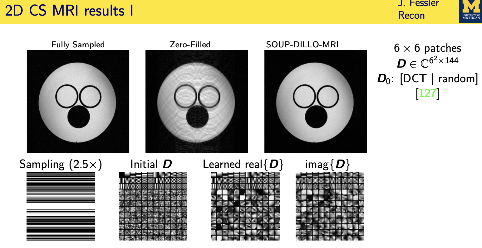
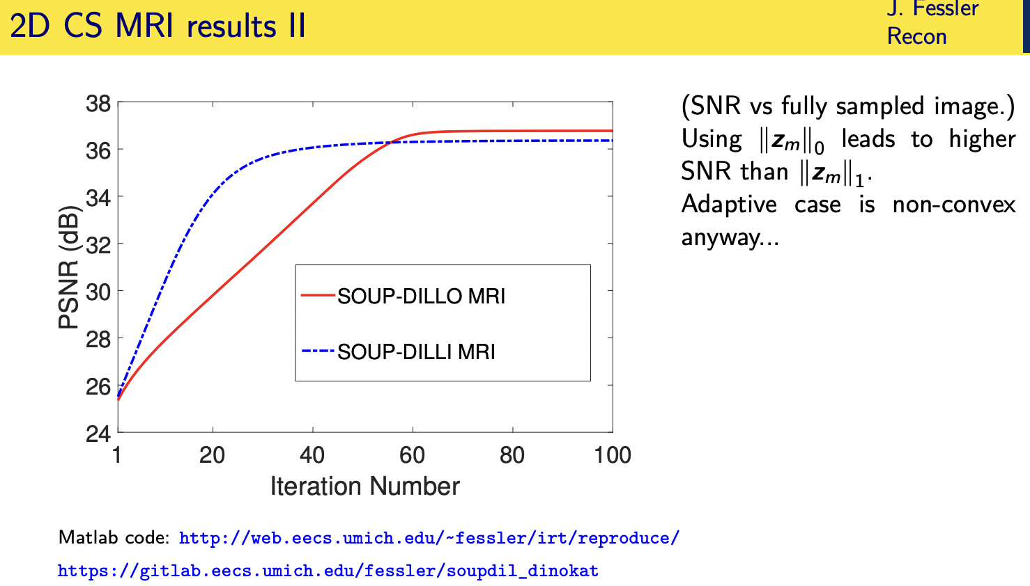
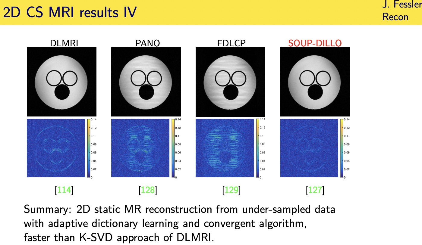
patient adaptive regularization— example:learned dictionary
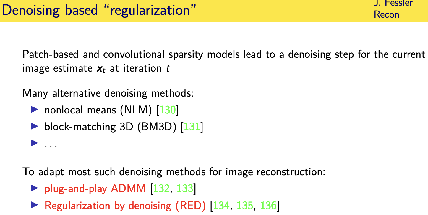
Denoising based “regularization”
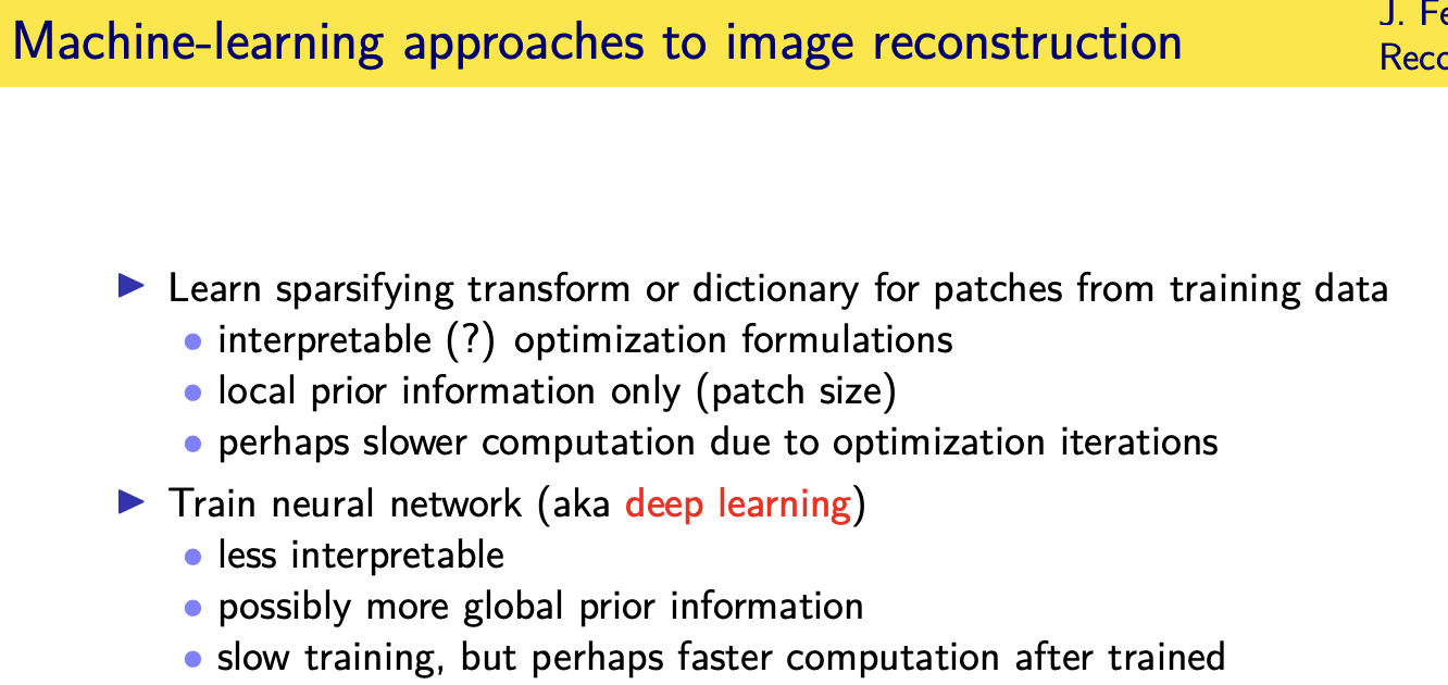
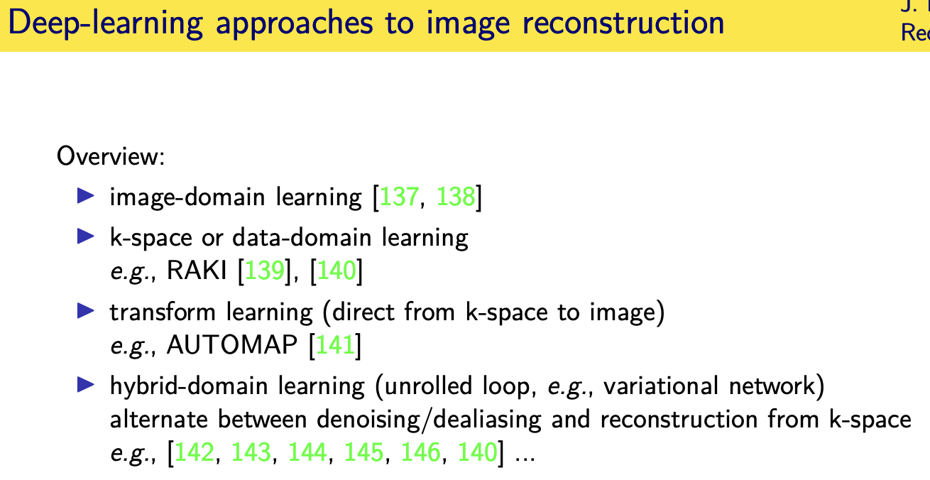
Deep- learning approaches for image reconstruction

Unrolled / unfolded loops
Challenges and limitations
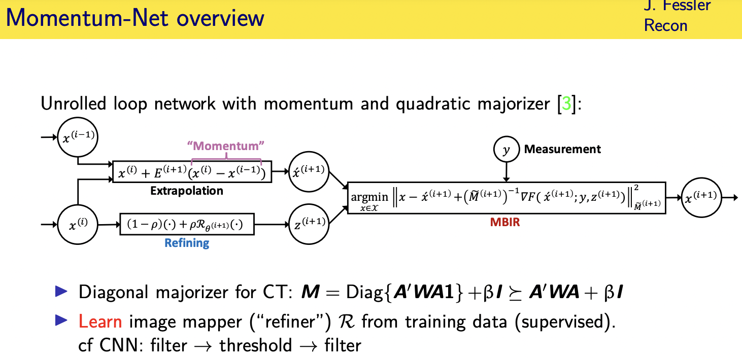
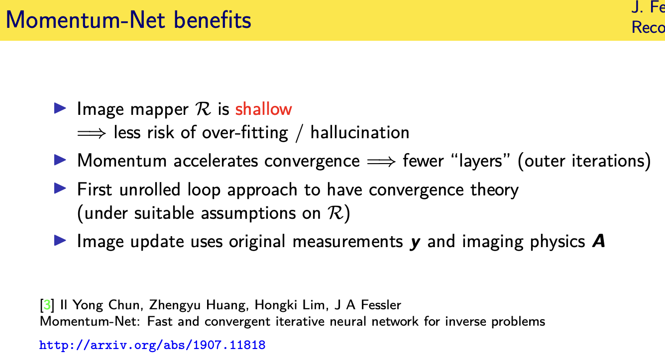
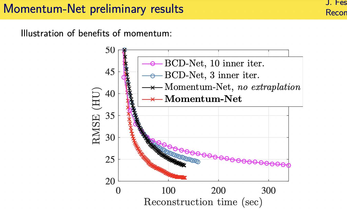
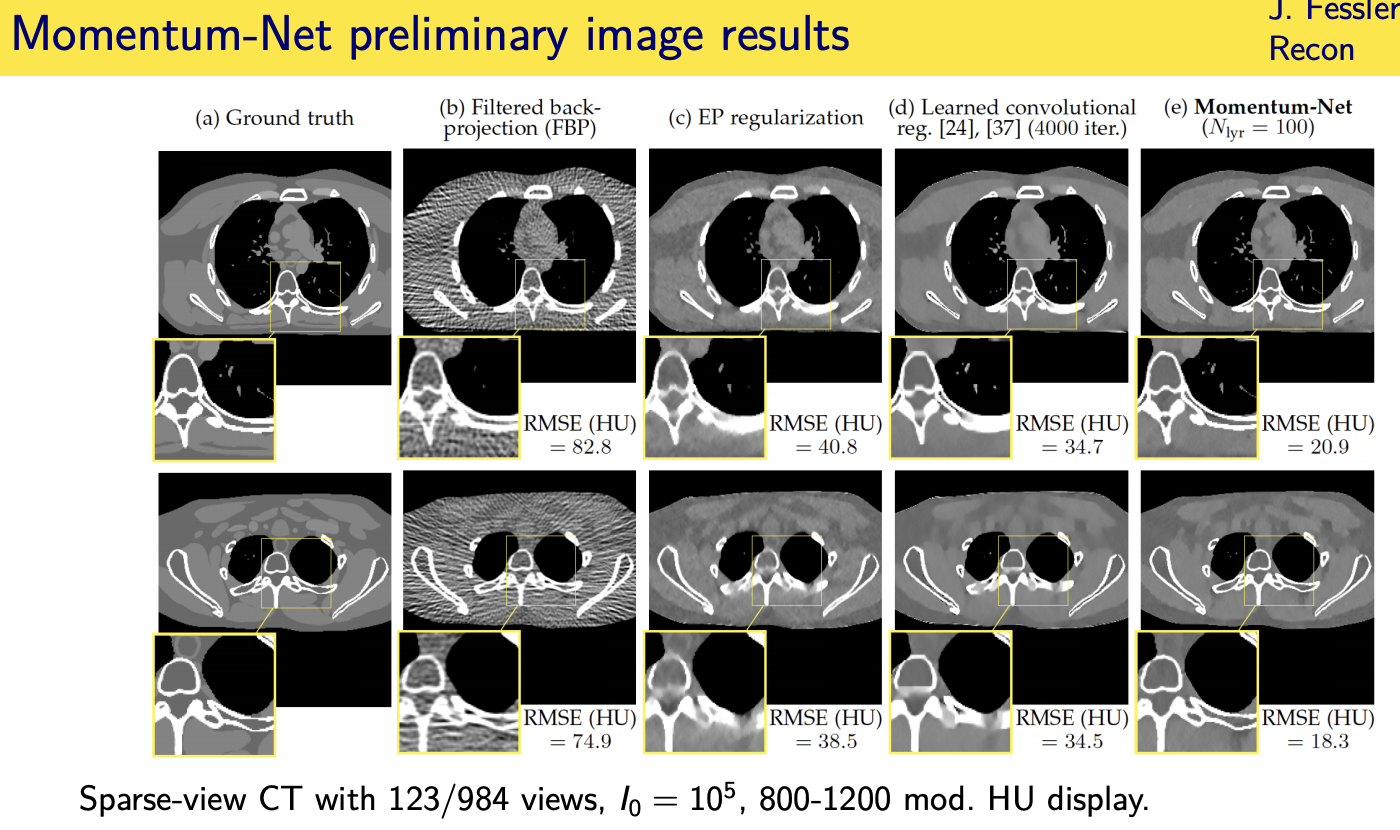
Momentum-Net
Looking forward
Acknowledgements
Code: https://github.com/JeffFessler/MIRT.jl
[1] S. Ravishankar, J. C. Ye, and J. A. Fessler. “Image reconstruction: from sparsity to data-adaptive methods and machine learning.” In:
Proc. IEEE 108.1 (Jan. 2020), 86–109. doi: 10.1109/JPROC.2019.2936204 (cit. on p. 2).
[2] J. A. Fessler. “Optimization methods for MR image reconstruction.” In: IEEE Sig. Proc. Mag. 37.1 (Jan. 2020), 33–40. doi:
10.1109/MSP.2019.2943645 (cit. on p. 2).
[3] I. Y. Chun et al. Momentum-Net: Fast and convergent iterative neural network for inverse problems. 2019. url:
http://arxiv.org/abs/1907.11818 (cit. on pp. 2, 85, 97, 98).
[4] M. K. Stehling, R. Turner, and P. Mansfield. “Echo-planar imaging: magnetic resonance imaging in a fraction of a second.” In: Science
254.5028 (Oct. 1991), 43–50. doi: 10.1126/science.1925560 (cit. on p. 5).
[5] P. Mansfield, R. Coxon, and J. Hykin. “Echo-volumar imaging (EVI) of the brain at 3.0 T: first normal volunteer and functional imaging
results.” In: J. Comp. Assisted Tomo. 19.6 (Nov. 1995), 847–52 (cit. on p. 5).
[6] A. Macovski. “Volumetric NMR imaging with time-varying gradients.” In: Mag. Res. Med. 2.1 (Feb. 1985), 29–40. doi:
10.1002/mrm.1910020105 (cit. on p. 5).
[7] C. H. Meyer et al. “Fast spiral coronary artery imaging.” In: Mag. Res. Med. 28.2 (Dec. 1992), 202–13. doi: 10.1002/mrm.1910280204
(cit. on p. 5).
[8] D. A. Feinberg et al. “Halving MR imaging time by conjugation: demonstration at 3.5 kG.” In: Radiology 161.2 (Nov. 1986), 527–31.
doi: 10.1148/radiology.161.2.3763926 (cit. on p. 5).
[9] P. Margosian, F. Schmitt, and D. E. Purdy. “Faster MR imaging: Imaging with half the data.” In: Health Care Instrum. 1.6 (1986),
195–7 (cit. on p. 5).
[10] D. C. Noll, D. G. Nishimura, and A. Macovski. “Homodyne detection in magnetic resonance imaging.” In: IEEE Trans. Med. Imag. 10.2
(June 1991), 154–63. doi: 10.1109/42.79473 (cit. on p. 5).
[11] J. W. Carlson. “An algorithm for NMR imaging reconstruction based on multiple RF receiver coils.” In: J. Mag. Res. 74.2 (Sept. 1987),
376–80. doi: ’10.1016/0022-2364(87)90348-9’ (cit. on p. 5).
[12] M. Hutchinson and U. Raff. “Fast MRI data acquisition using multiple detectors.” In: Mag. Res. Med. 6.1 (Jan. 1988), 87–91. doi:
10.1002/mrm.1910060110 (cit. on p. 5).
[13] P. B. Roemer et al. “The NMR phased array.” In: Mag. Res. Med. 16.2 (Nov. 1990), 192–225. doi: 10.1002/mrm.1910160203 (cit. on
pp. 5, 13).
[14] J. B. Ra and C. Y. Rim. “Fast imaging using subencoding data sets from multiple detectors.” In: Mag. Res. Med. 30.1 (July 1993),
142–5. doi: 10.1002/mrm.1910300123 (cit. on p. 5).
[15] D. K. Sodickson and W. J. Manning. “Simultaneous acquisition of spatial harmonics (SMASH): Fast imaging with radiofrequency coil
arrays.” In: Mag. Res. Med. 38.4 (Oct. 1997), 591–603. doi: 10.1002/mrm.1910380414 (cit. on p. 5).
[16] K. P. Pruessmann et al. “SENSE: sensitivity encoding for fast MRI.” In: Mag. Res. Med. 42.5 (Nov. 1999), 952–62. doi:
’10.1002/(SICI)1522-2594(199911)42:5<952::AID-MRM16>3.0.CO;2-S’ (cit. on pp. 5, 10, 13).
[17] K. P. Pruessmann et al. “Advances in sensitivity encoding with arbitrary k-space trajectories.” In: Mag. Res. Med. 46.4 (Oct. 2001),
638–51. doi: 10.1002/mrm.1241 (cit. on pp. 5, 14).
[18] M. A. Griswold et al. “Generalized autocalibrating partially parallel acquisitions (GRAPPA).” In: Mag. Res. Med. 47.6 (June 2002),
1202–10. doi: 10.1002/mrm.10171 (cit. on pp. 5, 37).
[19] Y. Cao and D. N. Levin. “Feature-recognizing MRI.” In: Mag. Res. Med. 30.3 (Sept. 1993), 305–17. doi: 10.1002/mrm.1910300306
(cit. on p. 5).
[20] N. Chauffert et al. “Variable density sampling with continuous trajectories.” In: SIAM J. Imaging Sci. 7.4 (2014), 1962–92. doi:
10.1137/130946642 (cit. on p. 5).
[21] C. Boyer et al. “On the generation of sampling schemes for magnetic resonance imaging.” In: SIAM J. Imaging Sci. 9.4 (2016), 2039–72.
doi: 10.1137/16m1059205 (cit. on p. 5).
[22] N. Chauffert et al. “A projection algorithm for gradient waveforms design in magnetic resonance imaging.” In: IEEE Trans. Med. Imag.
35.9 (Sept. 2016), 2026–39. doi: 10.1109/tmi.2016.2544251 (cit. on p. 5).
[23] C. Lazarus et al. “SPARKLING: variable-density k-space filling curves for accelerated T2*-weighted MRI.” In: Mag. Res. Med. 81.6 (June
2019), 3643–61. doi: 10.1002/mrm.27678 (cit. on p. 5).
[24] S. Ravishankar and Y. Bresler. “Adaptive sampling design for compressed sensing MRI.” In: Proc. Int’l. Conf. IEEE Engr. in Med. and
Biol. Soc. 2011, 3751–5. doi: 10.1109/IEMBS.2011.6090639 (cit. on p. 5).
[25] L. Baldassarre et al. “Learning-based compressive subsampling.” In: IEEE J. Sel. Top. Sig. Proc. 10.4 (June 2016), 809–22. doi:
10.1109/jstsp.2016.2548442 (cit. on pp. 5, 107).
[26] G. Godaliyadda et al. “A framework for dynamic image sampling based on supervised learning.” In: IEEE Trans. Computational Imaging
4.1 (Mar. 2018), 1–16. doi: 10.1109/tci.2017.2777482 (cit. on p. 5).
[27] C. D. Bahadir, A. V. Dalca, and M. R. Sabuncu. “Learning-based optimization of the under-sampling pattern in MRI.” In: Information
Processing in Medical Im. 2019, 780–92. doi: 10.1007/978-3-030-20351-1_61 (cit. on p. 5).
[28] H. K. Aggarwal and M. Jacob. “Joint optimization of sampling pattern and priors in model based deep learning.” In: Proc. IEEE Intl.
Symp. Biomed. Imag. 2020, 926–9. doi: 10.1109/ISBI45749.2020.9098639 (cit. on p. 5).
[29] E. Candes et al. “Image reconstruction from highly undersampled data using total variation minimization.” In: MRA Workshop, Oct. 8,
London Ontario. 2004, p. 147 (cit. on p. 5).
[30] M. Lustig et al. “Faster imaging with randomly perturbed, undersampled spirals and |L|1 reconstruction.” In: Proc. Intl. Soc. Mag. Res.
Med. 2005, p. 685. url: http://cds.ismrm.org/ismrm-2005/Files/00685.pdf (cit. on p. 5).
[31] S. J. LaRoque, E. Y. Sidky, and X. Pan. “Image Reconstruction from Sparse Data in Echo-Planar Imaging.” In: Proc. IEEE Nuc. Sci.
Symp. Med. Im. Conf. Vol. 5. 2006, 3166–9. doi: 10.1109/NSSMIC.2006.356547 (cit. on p. 5).
[32] M. Lustig, D. L. Donoho, and J. M. Pauly. “Rapid MR imaging with "compressed sensing" and randomly under-sampled 3DFT
trajectories.” In: Proc. Intl. Soc. Mag. Res. Med. 2006, p. 695. url: http://dev.ismrm.org//2006/0695.html (cit. on p. 5).
[33] K. T. Block, M. Uecker, and J. Frahm. “Undersampled radial MRI with multiple coils. Iterative image reconstruction using a total
variation constraint.” In: Mag. Res. Med. 57.6 (June 2007), 1086–98. doi: 10.1002/mrm.21236 (cit. on pp. 5, 27).
[34] E. Candes and J. Romberg. “Sparsity and incoherence in compressive sampling.” In: Inverse Prob. 23.3 (June 2007), 969–86. doi:
10.1088/0266-5611/23/3/008 (cit. on p. 5).
[35] M. Lustig, D. Donoho, and J. M. Pauly. “Sparse MRI: The application of compressed sensing for rapid MR imaging.” In: Mag. Res. Med.
58.6 (Dec. 2007), 1182–95. doi: 10.1002/mrm.21391 (cit. on pp. 5, 10, 94).
[36] J. C. Ye et al. “Projection reconstruction MR imaging using FOCUSS.” In: Mag. Res. Med. 57.4 (Apr. 2007), 764–75. doi:
10.1002/mrm.21202 (cit. on pp. 5, 29).
[37] E. J. Candes and M. B. Wakin. “An introduction to compressive sampling.” In: IEEE Sig. Proc. Mag. 25.2 (Mar. 2008), 21–30. doi:
10.1109/MSP.2007.914731 (cit. on p. 5).
[38] M. Lustig et al. “Compressed sensing MRI.” In: IEEE Sig. Proc. Mag. 25.2 (Mar. 2008), 72–82. doi: 10.1109/MSP.2007.914728 (cit. on
pp. 5, 27).
[39] FDA. 510k premarket notification of HyperSense (GE Medical Systems). 2017. url:
https://www.accessdata.fda.gov/scripts/cdrh/cfdocs/cfpmn/pmn.cfm?ID=K162722 (cit. on p. 5).
[40] FDA. 510k premarket notification of Compressed Sensing Cardiac Cine (Siemens). 2017. url:
https://www.accessdata.fda.gov/scripts/cdrh/cfdocs/cfpmn/pmn.cfm?ID=K163312 (cit. on p. 5).
[41] FDA. 510k premarket notification of Compressed SENSE. 2018. url:
https://www.accessdata.fda.gov/cdrh_docs/pdf17/K173079.pdf (cit. on p. 5).
[42] L. Geerts-Ossevoort et al. Compressed SENSE. Philips white paper 4522 991 31821 Nov. 2018. 2018. url:
https://philipsproductcontent.blob.core.windows.net/assets/20180109/619119731f2a42c4acd4a863008a46c7.pdf (cit. on
p. 5).
[43] G. Harikumar, C. Couvreur, and Y. Bresler. “Fast optimal and suboptimal algorithms for sparse solutions to linear inverse problems.” In:
Proc. IEEE Conf. Acoust. Speech Sig. Proc. Vol. 3. 1998, 1877–80. doi: 10.1109/ICASSP.1998.681830 (cit. on p. 5).
[44] J. Hamilton, D. Franson, and N. Seiberlich. “Recent advances in parallel imaging for MRI.” In: Prog. in Nuclear Magnetic Resonance
Spectroscopy 101 (Aug. 2017), 71–95. doi: 10.1016/j.pnmrs.2017.04.002.
[45] P. J. Shin et al. “Calibrationless parallel imaging reconstruction based on structured low-rank matrix completion.” In: Mag. Res. Med.
72.4 (Oct. 2014), 959–70. doi: 10.1002/mrm.24997 (cit. on pp. 6, 38).
[46] A. Balachandrasekaran, M. Mani, and M. Jacob. Calibration-free B0 correction of EPI data using structured low rank matrix recovery.
2018. url: http://arxiv.org/abs/1804.07436 (cit. on pp. 6, 38).
[47] J. P. Haldar and K. Setsompop. “Linear predictability in MRI reconstruction: Leveraging shift-invariant Fourier structure for faster and
better imaging.” In: IEEE Sig. Proc. Mag. 37.1 (Jan. 2020), 69–82. doi: 10.1109/MSP.2019.2949570 (cit. on p. 6).
[48] H-L. M. Cheng et al. “Practical medical applications of quantitative MR relaxometry.” In: J. Mag. Res. Im. 36.4 (Oct. 2012), 805–24.
doi: 10.1002/jmri.23718 (cit. on p. 6).
[49] B. Zhao, F. Lam, and Z-P. Liang. “Model-based MR parameter mapping with sparsity constraints: parameter estimation and
performance bounds.” In: IEEE Trans. Med. Imag. 33.9 (Sept. 2014), 1832–44. doi: 10.1109/TMI.2014.2322815 (cit. on p. 6).
[50] G. Nataraj et al. “Dictionary-free MRI PERK: Parameter estimation via regression with kernels.” In: IEEE Trans. Med. Imag. 37.9 (Sept.
2018), 2103–14. doi: 10.1109/TMI.2018.2817547 (cit. on p. 6).
[51] B. B. Mehta et al. “Magnetic resonance fingerprinting: a technical review.” In: Mag. Res. Med. 81.1 (Jan. 2019), 25–46. doi:
10.1002/mrm.27403 (cit. on p. 6).
[52] J. Bezanson et al. “Julia: A fresh approach to numerical computing.” In: SIAM Review 59.1 (2017), 65–98. doi: 10.1137/141000671
(cit. on p. 7).
[53] G. A. Wright. “Magnetic resonance imaging.” In: IEEE Sig. Proc. Mag. 14.1 (Jan. 1997), 56–66. doi: 10.1109/79.560324.
[54] M. Doneva. “Mathematical models for magnetic resonance imaging reconstruction: an overview of the approaches, problems, and future
research areas.” In: IEEE Sig. Proc. Mag. 37.1 (Jan. 2020), 24–32. doi: 10.1109/MSP.2019.2936964.
[55] J. A. Fessler. “Model-based image reconstruction for MRI.” In: IEEE Sig. Proc. Mag. 27.4 (July 2010). Invited submission to special issue
on medical imaging, 81–9. doi: 10.1109/MSP.2010.936726 (cit. on p. 11).
[56] J. A. Fessler and B. P. Sutton. “Nonuniform fast Fourier transforms using min-max interpolation.” In: IEEE Trans. Sig. Proc. 51.2 (Feb.
2003), 560–74. doi: 10.1109/TSP.2002.807005 (cit. on p. 10).
[57] B. P. Sutton, D. C. Noll, and J. A. Fessler. “Fast, iterative image reconstruction for MRI in the presence of field inhomogeneities.” In:
IEEE Trans. Med. Imag. 22.2 (Feb. 2003), 178–88. doi: 10.1109/TMI.2002.808360 (cit. on pp. 10, 14).
[58] A. Macovski. “Noise in MRI.” In: Mag. Res. Med. 36.3 (Sept. 1996), 494–7. doi: 10.1002/mrm.1910360327 (cit. on p. 11).
[59] J. A. Fessler et al. “Toeplitz-based iterative image reconstruction for MRI with correction for magnetic field inhomogeneity.” In: IEEE
Trans. Sig. Proc. 53.9 (Sept. 2005), 3393–402. doi: 10.1109/TSP.2005.853152 (cit. on p. 14).
[60] R. H. Chan and M. K. Ng. “Conjugate gradient methods for Toeplitz systems.” In: SIAM Review 38.3 (Sept. 1996), 427–82. doi:
10.1137/S0036144594276474 (cit. on p. 14).
[61] S. Ramani and J. A. Fessler. “Parallel MR image reconstruction using augmented Lagrangian methods.” In: IEEE Trans. Med. Imag. 30.3
(Mar. 2011), 694–706. doi: 10.1109/TMI.2010.2093536 (cit. on pp. 14, 30, 33).
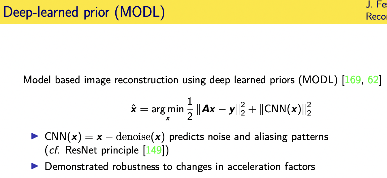
[62] H. K. Aggarwal, M. P. Mani, and M. Jacob. “MoDL: model-based deep learning architecture for inverse problems.” In: IEEE Trans. Med.
Imag. 38.2 (Feb. 2019), 394–405. doi: 10.1109/tmi.2018.2865356 (cit. on pp. 14, 85, 91).
[63] R. Boubertakh et al. “Non-quadratic convex regularized reconstruction of MR images from spiral acquisitions.” In: Signal Processing 86.9
(Sept. 2006), 2479–94. doi: 10.1016/j.sigpro.2005.11.011 (cit. on p. 15).
[64] S. Husse, Y. Goussard, and M. Idiert. “Extended forms of Geman & Yang algorithm: application to MRI reconstruction.” In: Proc. IEEE
Conf. Acoust. Speech Sig. Proc. Vol. 3. 2004, 513–16. doi: 10.1109/ICASSP.2004.1326594 (cit. on p. 15).
[65] A. Florescu et al. “A majorize-minimize memory gradient method for complex-valued inverse problems.” In: Signal Processing 103 (Oct.
2014), 285–95. doi: 10.1016/j.sigpro.2013.09.026 (cit. on pp. 15, 16).
[66] S. Geman and D. Geman. “Stochastic relaxation, Gibbs distributions, and Bayesian restoration of images.” In: IEEE Trans. Patt. Anal.
Mach. Int. 6.6 (Nov. 1984), 721–41. doi: 10.1109/TPAMI.1984.4767596 (cit. on p. 15).
[67] J. Besag. “On the statistical analysis of dirty pictures.” In: J. Royal Stat. Soc. Ser. B 48.3 (1986), 259–302. url:
http://www.jstor.org/stable/2345426 (cit. on p. 15).
[68] D. Kim and J. A. Fessler. “Optimized first-order methods for smooth convex minimization.” In: Mathematical Programming 159.1 (Sept.
2016), 81–107. doi: 10.1007/s10107-015-0949-3 (cit. on p. 16).
[69] Y. Drori. “The exact information-based complexity of smooth convex minimization.” In: J. Complexity 39 (Apr. 2017), 1–16. doi:
10.1016/j.jco.2016.11.001 (cit. on p. 16).
[70] Y. Nesterov. “A method of solving a convex programming problem with convergence rate O(1/k
2
).” In: Soviet Math. Dokl. 27.2 (1983),
372–76. url: http://www.core.ucl.ac.be/~nesterov/Research/Papers/DAN83.pdf (cit. on p. 16).
[71] Y. Drori and A. B. Taylor. “Efficient first-order methods for convex minimization: a constructive approach.” In: Mathematical
Programming (2020). doi: 10.1007/s10107-019-01410-2 (cit. on p. 16).
[72] F. Knoll et al. “Advancing machine learning for MR image reconstruction with an open competition: Overview of the 2019 fastMRI
challenge.” In: Mag. Res. Med. (2020). doi: 10.1002/mrm.28338 (cit. on p. 19).
[73] R. Tibshirani. “Regression shrinkage and selection via the LASSO.” In: J. Royal Stat. Soc. Ser. B 58.1 (1996), 267–88. url:
http://www.jstor.org/stable/2346178 (cit. on p. 21).
[74] E. J. Candes and Y. Plan. “Near-ideal model selection by `1 minimization.” In: Ann. Stat. 37.5a (2009), 2145–77. doi:
10.1214/08-AOS653 (cit. on p. 21).
[75] A. B. Taylor, J. M. Hendrickx, and Francois Glineur. “Exact worst-case performance of first-order methods for composite convex
optimization.” In: SIAM J. Optim. 27.3 (Jan. 2017), 1283–313. doi: 10.1137/16m108104x (cit. on pp. 21, 24, 25).
[76] D. Kim and J. A. Fessler. “Adaptive restart of the optimized gradient method for convex optimization.” In: J. Optim. Theory Appl. 178.1
(July 2018), 240–63. doi: 10.1007/s10957-018-1287-4 (cit. on pp. 21, 24, 25).
[77] I. Daubechies, M. Defrise, and C. De Mol. “An iterative thresholding algorithm for linear inverse problems with a sparsity constraint.” In:
Comm. Pure Appl. Math. 57.11 (Nov. 2004), 1413–57. doi: 10.1002/cpa.20042 (cit. on p. 23).
[78] P. Combettes and V. Wajs. “Signal recovery by proximal forward-backward splitting.” In: SIAM J. Multi. Mod. Sim. 4.4 (2005),
1168–200. doi: 10.1137/050626090 (cit. on p. 23).
[79] M. J. Muckley, D. C. Noll, and J. A. Fessler. “Fast parallel MR image reconstruction via B1-based, adaptive restart, iterative soft
thresholding algorithms (BARISTA).” In: IEEE Trans. Med. Imag. 34.2 (Feb. 2015), 578–88. doi: 10.1109/TMI.2014.2363034 (cit. on
p. 23).
[80] A. Beck and M. Teboulle. “A fast iterative shrinkage-thresholding algorithm for linear inverse problems.” In: SIAM J. Imaging Sci. 2.1
(2009), 183–202. doi: 10.1137/080716542 (cit. on p. 23).
[81] A. Beck and M. Teboulle. “Fast gradient-based algorithms for constrained total variation image denoising and deblurring problems.” In:
IEEE Trans. Im. Proc. 18.11 (Nov. 2009), 2419–34. doi: 10.1109/TIP.2009.2028250 (cit. on pp. 23, 28).
[82] L. El Gueddari et al. “Self-calibrating nonlinear reconstruction algorithms for variable density sampling and parallel reception MRI.” In:
Proc. IEEE SAM. 2018, 415–9. doi: 10.1109/SAM.2018.8448776 (cit. on p. 24).
[83] C. Y. Lin and J. A. Fessler. “Accelerated methods for low-rank plus sparse image reconstruction.” In: Proc. IEEE Intl. Symp. Biomed.
Imag. 2018, 48–51. doi: 10.1109/ISBI.2018.8363520 (cit. on p. 24).
[84] C. Y. Lin and J. A. Fessler. “Efficient dynamic parallel MRI reconstruction for the low-rank plus sparse model.” In: IEEE Trans.
Computational Imaging 5.1 (Mar. 2019), 17–26. doi: 10.1109/TCI.2018.2882089 (cit. on p. 24).
[85] Z. Ramzi, P. Ciuciu, and J-L. Starck. “Benchmarking proximal methods acceleration enhancements for CS-acquired MR image analysis
reconstruction.” In: Sig. Proc. with Adapt. Sparse Struct. Rep. SPARS. 2019. url: https://hal.inria.fr/hal-02298569 (cit. on
p. 24).
[86] B. O’Donoghue and E. Candes. “Adaptive restart for accelerated gradient schemes.” In: Found. Comp. Math. 15.3 (June 2015), 715–32.
doi: 10.1007/s10208-013-9150-3 (cit. on p. 24).
[87] J. Liang and C-B. Schonlieb. Faster FISTA. 2018. url: http://arxiv.org/abs/1807.04005 (cit. on p. 24).
[88] J. Liang and C-B. Schonlieb. Improving FISTA: Faster, smarter and greedier. 2018. url: http://arxiv.org/abs/1811.01430 (cit. on
p. 24).
[89] A. Chambolle. “An algorithm for total variation minimization and applications.” In: J. Math. Im. Vision 20.1-2 (Jan. 2004), 89–97. doi:
10.1023/B:JMIV.0000011325.36760.1e (cit. on p. 28).
[90] Y. Wang et al. “A new alternating minimization algorithm for total variation image reconstruction.” In: SIAM J. Imaging Sci. 1.3 (2008),
248–72. doi: 10.1137/080724265 (cit. on p. 29).
[91] T. Goldstein and S. Osher. “The split Bregman method for L1-regularized problems.” In: SIAM J. Imaging Sci. 2.2 (2009), 323–43. doi:
10.1137/080725891 (cit. on p. 30).
[92] J. Aelterman et al. “Augmented Lagrangian based reconstruction of non-uniformly sub-Nyquist sampled MRI data.” In: Signal Processing
91.12 (Jan. 2011), 2731–42. doi: 10.1016/j.sigpro.2011.04.033 (cit. on p. 30).
[93] J. Eckstein and D. P. Bertsekas. “On the Douglas-Rachford splitting method and the proximal point algorithm for maximal monotone
operators.” In: Mathematical Programming 55.1-3 (Apr. 1992), 293–318. doi: 10.1007/BF01581204 (cit. on p. 30).
[94] S. Boyd et al. “Distributed optimization and statistical learning via the alternating direction method of multipliers.” In: Found. & Trends
in Machine Learning 3.1 (2010), 1–122. doi: 10.1561/2200000016 (cit. on pp. 30, 32).
[95] Z. Xu, M. A. T. Figueiredo, and T. Goldstein. “Adaptive ADMM with spectral penalty parameter selection.” In: aistats. 2017, 718–27.
url: http://proceedings.mlr.press/v54/xu17a.html (cit. on p. 32).
[96] B. Wohlberg. ADMM penalty parameter selection by residual balancing. 2017. url: http://arxiv.org/abs/1704.06209 (cit. on p. 32).
[97] J. Eckstein. “Parallel alternating direction multiplier decomposition of convex programs.” In: J. Optim. Theory Appl. 80.1 (Jan. 1994),
39–62. doi: 10.1007/BF02196592 (cit. on p. 32).
[98] M. Le and J. A. Fessler. “Efficient, convergent SENSE MRI reconstruction for non-periodic boundary conditions via tridiagonal solvers.”
In: IEEE Trans. Computational Imaging 3.1 (Mar. 2017), 11–21. doi: 10.1109/TCI.2016.2626999 (cit. on pp. 32, 33).
[99] Y. Chen et al. “Fast algorithms for image reconstruction with application to partially parallel MR imaging.” In: SIAM J. Imaging Sci. 5.1
(2012), 90–118. doi: 10.1137/100792688 (cit. on pp. 33, 34).
[100] A. Chambolle and T. Pock. “A first-order primal-dual algorithm for convex problems with applications to imaging.” In: J. Math. Im.
Vision 40.1 (2011), 120–145. doi: 10.1007/s10851-010-0251-1 (cit. on p. 34).
[101] T. Pock and A. Chambolle. “Diagonal preconditioning for first order primal-dual algorithms in convex optimization.” In: Proc. Intl. Conf.
Comp. Vision. 2011, 1762–9. doi: 10.1109/ICCV.2011.6126441 (cit. on p. 34).
[102] P. L. Combettes and J. C. Pesquet. “Primal-dual splitting algorithm for solving inclusions with mixtures of composite, Lipschitzian, and
parallel-sum type monotone operators.” In: Set-Valued Var Anal 20.2 (June 2012), 307–30. doi: 10.1007/s11228-011-0191-y (cit. on
p. 34).
[103] L. Condat. “A primal-dual splitting method for convex optimization involving Lipschitzian, proximable and linear composite terms.” In: J.
Optim. Theory Appl. 158.2 (2013), 460–79. doi: 10.1007/s10957-012-0245-9 (cit. on p. 34).
[104] E. Y. Sidky, J. H. Jorgensen, and X. Pan. “Convex optimization problem prototyping for image reconstruction in computed tomography
with the Chambolle-Pock algorithm.” In: Phys. Med. Biol. 57.10 (May 2012), 3065–92. doi: 10.1088/0031-9155/57/10/3065 (cit. on
p. 34).
[105] B. Công Vu. “A splitting algorithm for dual monotone inclusions involving cocoercive operators.” In: Adv. in Comp. Math. 38.3 (Apr.
2013), 667–81. doi: 10.1007/s10444-011-9254-8 (cit. on p. 34).
[106] T. Valkonen. “A primal-dual hybrid gradient method for nonlinear operators with applications to MRI.” In: Inverse Prob. 30.5 (May
2014), p. 055012. doi: 10.1088/0266-5611/30/5/055012 (cit. on p. 34).
[107] F. Ong, M. Uecker, and M. Lustig. Accelerating non-Cartesian MRI reconstruction convergence using k-space preconditioning. 2019.
url: http://arxiv.org/abs/1902.09657 (cit. on p. 34).
[108] M. Lustig and J. M. Pauly. “SPIRiT: Iterative self-consistent parallel imaging reconstruction from arbitrary k-space.” In: Mag. Res. Med.
64.2 (Aug. 2010), 457–71. doi: 10.1002/mrm.22428 (cit. on pp. 37, 71).
[109] M. Murphy et al. “Fast `1-SPIRiT compressed sensing parallel imaging MRI: scalable parallel implementation and clinically feasible
runtime.” In: IEEE Trans. Med. Imag. 31.6 (June 2012), 1250–62. doi: 10.1109/TMI.2012.2188039 (cit. on p. 37).
[110] D. Weller, S. Ramani, and J. A. Fessler. “Augmented Lagrangian with variable splitting for faster non-Cartesian L1-SPIRiT MR image
reconstruction.” In: IEEE Trans. Med. Imag. 33.2 (Feb. 2014), 351–61. doi: 10.1109/TMI.2013.2285046 (cit. on p. 37).
[111] J. Duan, Y. Liu, and P. Jing. “Efficient operator splitting algorithm for joint sparsity-regularized SPIRiT-based parallel MR imaging
reconstruction.” In: Mag. Res. Im. 46 (Feb. 2018), 81–9. doi: 10.1016/j.mri.2017.10.013 (cit. on p. 37).
[112] M. Uecker et al. “ESPIRiT-an eigenvalue approach to autocalibrating parallel MRI: Where SENSE meets GRAPPA.” In: Mag. Res. Med.
71.3 (Mar. 2014), 990–1001. doi: 10.1002/mrm.24751 (cit. on p. 38).
[113] L. El Gueddari et al. “Calibrationless OSCAR-based image reconstruction in compressed sensing parallel MRI.” In: Proc. IEEE Intl. Symp.
Biomed. Imag. 2019, 1532–6 (cit. on p. 38).
[114] S. Ravishankar and Y. Bresler. “MR image reconstruction from highly undersampled k-space data by dictionary learning.” In: IEEE Trans.
Med. Imag. 30.5 (May 2011), 1028–41. doi: 10.1109/TMI.2010.2090538 (cit. on pp. 42, 51, 71, 72).
[115] S. Ravishankar and Y. Bresler. “Efficient blind compressed sensing using sparsifying transforms with convergence guarantees and
application to MRI.” In: SIAM J. Imaging Sci. 8.4 (2015), 2519–57. doi: 10.1137/141002293 (cit. on pp. 43, 51).
[116] I. Y. Chun and J. A. Fessler. “Convolutional dictionary learning: acceleration and convergence.” In: IEEE Trans. Im. Proc. 27.4 (Apr.
2018), 1697–712. doi: 10.1109/TIP.2017.2761545 (cit. on pp. 46, 48).
[117] I. Y. Chun and J. A. Fessler. Convolutional analysis operator learning: acceleration and convergence. 2018. url:
http://arxiv.org/abs/1802.05584 (cit. on pp. 46, 47).
[118] T. Nguyen-Duc and W-K. Jeong. “Compressed sensing dynamic MRI reconstruction using multi-scale 3D convolutional sparse coding
with elastic net regularization.” In: Proc. IEEE Intl. Symp. Biomed. Imag. 2018, 332–5. doi: 10.1109/ISBI.2018.8363586 (cit. on p. 46).
[119] B. Wohlberg. “Efficient algorithms for convolutional sparse representations.” In: IEEE Trans. Im. Proc. 25.1 (Jan. 2016), 301–15. doi:
10.1109/TIP.2015.2495260 (cit. on p. 46).
[120] A. Lahiri, S. Ravishankar, and J. A. Fessler. “Combining supervised and semi-blind dictionary (Super-BReD) learning for MRI
reconstruction.” In: Proc. Intl. Soc. Mag. Res. Med. To appear. 2020, p. 3456 (cit. on p. 51).
[121] G. Wang et al. “Image reconstruction is a new frontier of machine learning.” In: IEEE Trans. Med. Imag. 37.6 (June 2018), 1289–96.
doi: 10.1109/TMI.2018.2833635 (cit. on p. 52).
[122] M. Aharon, M. Elad, and A. Bruckstein. “K-SVD: an algorithm for designing overcomplete dictionaries for sparse representation.” In:
IEEE Trans. Sig. Proc. 54.11 (Nov. 2006), 4311–22. doi: 10.1109/TSP.2006.881199 (cit. on p. 58).
[123] S. Ravishankar and Y. Bresler. “l0 sparsifying transform learning with efficient optimal updates and convergence guarantees.” In: IEEE
Trans. Sig. Proc. 63.9 (May 2015), 2389–404. doi: 10.1109/TSP.2015.2405503 (cit. on p. 58).
[124] X. Zheng et al. “PWLS-ULTRA: An efficient clustering and learning-based approach for low-dose 3D CT image reconstruction.” In: IEEE
Trans. Med. Imag. 37.6 (June 2018), 1498–510. doi: 10.1109/TMI.2018.2832007 (cit. on pp. 60, 61, 64, 65).
[125] H. Nien and J. A. Fessler. “Relaxed linearized algorithms for faster X-ray CT image reconstruction.” In: IEEE Trans. Med. Imag. 35.4
(Apr. 2016), 1090–8. doi: 10.1109/TMI.2015.2508780 (cit. on p. 60).
[126] S. Ravishankar and Y. Bresler. “Data-driven learning of a union of sparsifying transforms model for blind compressed sensing.” In: IEEE
Trans. Computational Imaging 2.3 (Sept. 2016), 294–309. doi: 10.1109/TCI.2016.2567299 (cit. on pp. 63, 94).
[127] S. Ravishankar, R. R. Nadakuditi, and J. A. Fessler. “Efficient sum of outer products dictionary learning (SOUP-DIL) and its application
to inverse problems.” In: IEEE Trans. Computational Imaging 3.4 (Dec. 2017), 694–709. doi: 10.1109/TCI.2017.2697206 (cit. on
pp. 68, 69, 71, 72).
[128] X. Qu et al. “Magnetic resonance image reconstruction from undersampled measurements using a patch-based nonlocal operator.” In:
Med. Im. Anal. 18.6 (Aug. 2014), 843–56. doi: 10.1016/j.media.2013.09.007 (cit. on pp. 71, 72).
[129] Z. Zhan et al. “Fast multiclass dictionaries learning with geometrical directions in MRI reconstruction.” In: IEEE Trans. Biomed. Engin.
63.9 (Sept. 2016), 1850–61. doi: 10.1109/tbme.2015.2503756 (cit. on p. 72).
[130] A. Buades, B. Coll, and J-M. Morel. “The staircasing effect in neighborhood filters and its solution.” In: IEEE Trans. Im. Proc. 15.6
(June 2006), 1499–505. doi: 10.1109/TIP.2006.871137 (cit. on p. 74).
[131] K. Dabov et al. “Image denoising by sparse 3-D transform-domain collaborative filtering.” In: IEEE Trans. Im. Proc. 16.8 (Aug. 2007),
2080–95. doi: 10.1109/TIP.2007.901238 (cit. on p. 74).
[132] S. H. Chan, X. Wang, and O. A. Elgendy. “Plug-and-play ADMM for image restoration: fixed-point convergence and applications.” In:
IEEE Trans. Computational Imaging 3.1 (Mar. 2017), 84–98. doi: 10.1109/tci.2016.2629286 (cit. on p. 74).
[133] G. T. Buzzard et al. “Plug-and-play unplugged: optimization-free reconstruction using consensus equilibrium.” In: SIAM J. Imaging Sci.
11.3 (Jan. 2018), 2001–20. doi: 10.1137/17m1122451 (cit. on p. 74).
[134] Y. Romano, M. Elad, and P. Milanfar. “The little engine that could: Regularization by denoising (RED).” In: SIAM J. Imaging Sci. 10.4
(2017), 1804–44. doi: 10.1137/16M1102884 (cit. on p. 74).
[135] E. T. Reehorst and P. Schniter. Regularization by denoising: clarifications and new interpretations. 2018. url:
http://arxiv.org/abs/1806.02296 (cit. on p. 74).
[136] R. Ahmad et al. “Plug and play methods for magnetic resonance imaging.” In: IEEE Sig. Proc. Mag. 37.1 (Jan. 2020), 105–16. doi:
10.1109/MSP.2019.2949470 (cit. on p. 74).
[137] S. Wang et al. “Exploiting deep convolutional neural network for fast magnetic resonance imaging.” In: Proc. Intl. Soc. Mag. Res. Med.
2016, p. 1778. url: http://archive.ismrm.org/2016/1778.html (cit. on pp. 77, 81).
[138] D. Lee, J. Yoo, and J. C. Ye. Deep artifact learning for compressed sensing and parallel MRI. 2017. url:
http://arxiv.org/abs/1703.01120 (cit. on p. 77).
[139] M. Akcakaya et al. “Scan-specific robust artificial-neural-networks for k-space interpolation (RAKI) reconstruction: Database-free deep
learning for fast imaging.” In: Mag. Res. Med. 81.1 (Jan. 2019), 439–53. doi: 10.1002/mrm.27420 (cit. on p. 77).
[140] Y. Han and J. C. Ye. “K-space deep learning for accelerated MRI.” In: IEEE Trans. Med. Imag. 39.2 (Feb. 2020), 377–86. doi:
10.1109/TMI.2019.2927101 (cit. on p. 77).
[141] B. Zhu et al. “Image reconstruction by domain-transform manifold learning.” In: Nature 555 (Mar. 2018), 487–92. doi:
10.1038/nature25988 (cit. on p. 77).
[142] Y. Yang et al. “Deep ADMM-net for compressive sensing MRI.” In: Neural Info. Proc. Sys. 2016, 10–18. url:
https://papers.nips.cc/paper/6406-deep-admm-net-for-compressive-sensing-mri (cit. on pp. 77, 85).
[143] K. Hammernik et al. “Learning a variational network for reconstruction of accelerated MRI data.” In: Mag. Res. Med. 79.6 (June 2018),
3055–71. doi: 10.1002/mrm.26977 (cit. on pp. 77, 85).
[144] J. Schlemper et al. “A deep cascade of convolutional neural networks for dynamic MR image reconstruction.” In: IEEE Trans. Med. Imag.
37.2 (Feb. 2018), 491–503. doi: 10.1109/tmi.2017.2760978 (cit. on pp. 77, 102).
[145] T. M. Quan, T. Nguyen-Duc, and W-K. Jeong. “Compressed sensing MRI reconstruction using a generative adversarial network with a
cyclic loss.” In: IEEE Trans. Med. Imag. 37.6 (June 2018), 1488–97. doi: 10.1109/TMI.2018.2820120 (cit. on p. 77).
[146] D. Lee et al. “Deep residual learning for accelerated MRI using magnitude and phase networks.” In: IEEE Trans. Biomed. Engin. 65.9
(Sept. 2018), 1985–95. doi: 10.1109/TBME.2018.2821699 (cit. on p. 77).
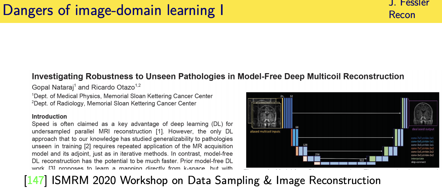
[147] G. Nataraj and R. Otazo. “Investigating robustness to unseen pathologies in model-free deep multicoil reconstruction.” In: ISMRM
Workshop on Data Sampling and Image Reconstruction. 2020 (cit. on p. 79).
[148] G. Yang et al. “DAGAN: Deep de-aliasing generative adversarial networks for fast compressed sensing MRI reconstruction.” In: IEEE
Trans. Med. Imag. 37.6 (June 2018), 1310–21. doi: 10.1109/TMI.2017.2785879 (cit. on p. 81).
[149] K. He et al. “Deep residual learning for image recognition.” In: Proc. IEEE Conf. on Comp. Vision and Pattern Recognition. 2016, 770–8.
doi: 10.1109/CVPR.2016.90 (cit. on pp. 81, 91).
[150] K. Zhang et al. “Beyond a Gaussian denoiser: residual learning of deep CNN for image denoising.” In: IEEE Trans. Im. Proc. 26.7 (July
2017), 3142–55. doi: 10.1109/tip.2017.2662206 (cit. on p. 81).
[151] K. Gregor and Y. LeCun. “Learning fast approximations of sparse coding.” In: Proc. Intl. Conf. Mach. Learn. 2010. url:
http://yann.lecun.com/exdb/publis/pdf/gregor-icml-10.pdf (cit. on p. 85).
[152] T. Meinhardt et al. “Learning proximal operators: using denoising networks for regularizing inverse imaging problems.” In: Proc. Intl.
Conf. Comp. Vision. 2017, 1799–808. doi: 10.1109/ICCV.2017.198 (cit. on p. 85).
[153] U. Schmidt and S. Roth. “Shrinkage fields for effective image restoration.” In: Proc. IEEE Conf. on Comp. Vision and Pattern
Recognition. 2014, 2774–81. doi: 10.1109/CVPR.2014.349 (cit. on p. 85).
[154] Y. Chen, W. Yu, and T. Pock. “On learning optimized reaction diffusion processes for effective image restoration.” In: Proc. IEEE Conf.
on Comp. Vision and Pattern Recognition. 2015, 5261–9. doi: 10.1109/CVPR.2015.7299163 (cit. on p. 85).
[155] Y. Chen and T. Pock. “Trainable nonlinear reaction diffusion: A flexible framework for fast and effective image restoration.” In: IEEE
Trans. Patt. Anal. Mach. Int. 39.6 (June 2017), 1256–72. doi: 10.1109/TPAMI.2016.2596743 (cit. on p. 85).
[156] K. Hammernik et al. “Learning a variational model for compressed sensing MRI reconstruction.” In: Proc. Intl. Soc. Mag. Res. Med.
2016, p. 1088. url: http://archive.ismrm.org/2016/1088.html (cit. on p. 85).
[157] Y. Yang et al. ADMM-net: A deep learning approach for compressive sensing MRI. 2017. url: http://arxiv.org/abs/1705.06869
(cit. on p. 85).
[158] B. Xin et al. Maximal sparsity with deep networks? 2016. url: http://arxiv.org/abs/1605.01636 (cit. on p. 85).
[159] P. Schniter. “Recent advances in approximate message passing.” In: spars-17. 2017, plenary (cit. on p. 85).
[160] H-Y. Liu et al. “Compressive imaging with iterative forward models.” In: Proc. IEEE Conf. Acoust. Speech Sig. Proc. 2017 (cit. on p. 85).
[161] J. Adler and O. Oktem. “Learned primal-dual reconstruction.” In: IEEE Trans. Med. Imag. 37.6 (June 2018), 1322–32. doi:
10.1109/tmi.2018.2799231 (cit. on p. 85).
[162] Y. Malitsky and T. Pock. “A first-order primal-dual algorithm with linesearch.” In: SIAM J. Optim. 28.1 (Jan. 2018), 411–32. doi:
10.1137/16m1092015 (cit. on p. 85).
[163] S. Ravishankar et al. “Deep dictionary-transform learning for image reconstruction.” In: Proc. IEEE Intl. Symp. Biomed. Imag. 2018,
1208–12. doi: 10.1109/ISBI.2018.8363788 (cit. on pp. 85, 93).
[164] I. Y. Chun and J. A. Fessler. “Deep BCD-net using identical encoding-decoding CNN structures for iterative image recovery.” In: Proc.
IEEE Wkshp. on Image, Video, Multidim. Signal Proc. 2018, 1–5. doi: 10.1109/IVMSPW.2018.8448694 (cit. on p. 85).
[165] I. Y. Chun and J. A. Fessler. Deep BCD-net using identical encoding-decoding CNN structures for iterative image recovery. 2018. url:
http://arxiv.org/abs/1802.07129 (cit. on p. 85).
[166] H. Lim et al. “Application of trained deep BCD-net to iterative low-count PET image reconstruction.” In: Proc. IEEE Nuc. Sci. Symp.
Med. Im. Conf. 2018, 1–4. doi: 10.1109/NSSMIC.2018.8824563 (cit. on p. 85).
[167] I. Y. Chun et al. “Fast and convergent iterative image recovery using trained convolutional neural networks.” In: Allerton Conf. on
Comm., Control, and Computing. Invited. 2018, 155–9. doi: 10.1109/ALLERTON.2018.8635932 (cit. on p. 85).
[168] J. R. Hershey, J. L. Roux, and F. Weninger. Deep unfolding: Model-based inspiration of novel deep architectures. 2014. url:
http://arxiv.org/abs/1409.2574 (cit. on p. 85).
[169] H. K. Aggarwal, M. P. Mani, and M. Jacob. “Model based image reconstruction using deep learned priors (MODL).” In: Proc. IEEE Intl.
Symp. Biomed. Imag. 2018, 671–4. doi: 10.1109/ISBI.2018.8363663 (cit. on pp. 85, 91).
[170] K. H. Jin, M. McCann, and M. Unser. “BPConvNet for compressed sensing recovery in bioimaging.” In: spars-17. 2017 (cit. on p. 85).
[171] H. Chen et al. “LEARN: Learned experts: assessment-based reconstruction network for sparse-data CT.” In: IEEE Trans. Med. Imag. 37.6
(June 2018), 1333–47. doi: 10.1109/TMI.2018.2805692 (cit. on p. 85).
[172] D. Wu et al. End-to-end abnormality detection in medical imaging. 2018. url: http://arxiv.org/abs/1711.02074 (cit. on p. 85).
[173] D. Liang et al. “Deep MRI reconstruction: Unrolled optimization algorithms meet neural networks.” In: IEEE Sig. Proc. Mag. 37.1 (Jan.
2020), 141–51. doi: 10.1109/MSP.2019.2950557 (cit. on p. 85).
[174] V. Monga, Y. Li, and Y. C. Eldar. Algorithm unrolling: interpretable, efficient deep learning for signal and image processing. 2020. url:
http://arxiv.org/abs/1912.10557 (cit. on p. 85).
[175] I. J. Goodfellow et al. Generative adversarial networks. 2014. url: http://arxiv.org/abs/1406.2661 (cit. on pp. 86, 87).
[176] X. Chen et al. “InfoGAN: interpretable representation learning by information maximizing generative adversarial nets.” In: Neural Info.
Proc. Sys. 2016, 2172–80. url: https://papers.nips.cc/paper/6399-infogan-interpretable-representation-learning-byinformation-maximizing-generative-adversarial-nets (cit. on pp. 86, 87).
[177] A. Bora et al. “Compressed sensing using generative models.” In: Proc. Intl. Conf. Mach. Learn. Vol. 70. 2017, 537–46. url:
http://proceedings.mlr.press/v70/bora17a.html (cit. on pp. 86, 87).
[178] S. Kolouri et al. Sliced-Wasserstein autoencoder: an embarrassingly simple generative model. 2018. url:
http://arxiv.org/abs/1804.01947 (cit. on p. 88).
[179] D. Berthelot, T. Schumm, and L. Metz. BEGAN: boundary equilibrium generative adversarial networks. 2017. url:
http://arxiv.org/abs/1703.10717 (cit. on pp. 89, 90).
[180] B. Yaman et al. “Self-supervised learning of physics-based reconstruction neural networks without fully-sampled reference data.” In: Mag.
Res. Med. (2020). doi: 10.1002/mrm.28378 (cit. on p. 92).
[181] V. Antun et al. On instabilities of deep learning in image reconstruction - Does AI come at a cost? 2019. url:
http://arxiv.org/abs/1902.05300 (cit. on p. 92).
[182] E. Haneda et al. “CT sinogram analysis using deep learning.” In: Proc. 5th Intl. Mtg. on Image Formation in X-ray CT. 2018, 419–22
(cit. on p. 105).
[183] Q. De Man et al. “A two-dimensional feasibility study of deep learning-based feature detection and characterization directly from CT
sinograms.” In: Med. Phys. 46.12 (Dec. 2019), e790–800. doi: 10.1002/mp.13640 (cit. on p. 105).
[184] B. Gozcu et al. “Learning-based compressive MRI.” In: IEEE Trans. Med. Imag. 37.6 (June 2018), 1394–406. doi:
10.1109/TMI.2018.2832540 (cit. on p. 107).


 被折叠的 条评论
为什么被折叠?
被折叠的 条评论
为什么被折叠?
 到【灌水乐园】发言


