


这是学习笔记的第 2025 篇文章
有这样一个需求,是需要根据一些动漫的信息来做出一些数据分析,大概有1700多部动漫作品,相关的属性有差不多20个。
这种情况下,看是看不出来的,我们得有一定的方法论来处理,这里我就使用主成分分析法来做。
1.环境准备
openxlsx
psych
VIM(选用)
scatterplot3d(选用)
2.数据清洗和整理
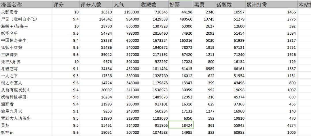
数据框包含1714个样本,20个变量,我们对数据清洗和整理。
序号 | 变量 | 序号 | 变量 |
1 | 漫画名称 | 11 | 是否完结 |
2 | 标签 | 12 | 更新时间 |
3 | 作者 | 13 | 话题数 |
4 | 合约关系 | 14 | 累计打赏 |
5 | 评分 | 15 | 本站打赏排名 |
6 | 评分人数 | 16 | 今日打赏数 |
7 | 人气 | 17 | 本月月票 |
8 | 收藏数 | 18 | 本月打赏排名 |
9 | 好票 | 19 | 单次得到打赏最高数额 |
10 | 黑票 | 20 | 作者作品数 |
首先需要做数据清洗,其中列“标签”,“作者”,“合约关系”,“是否完结”,“更新时间”的数据值为文本和时间类型,不适合做数值计算分析。

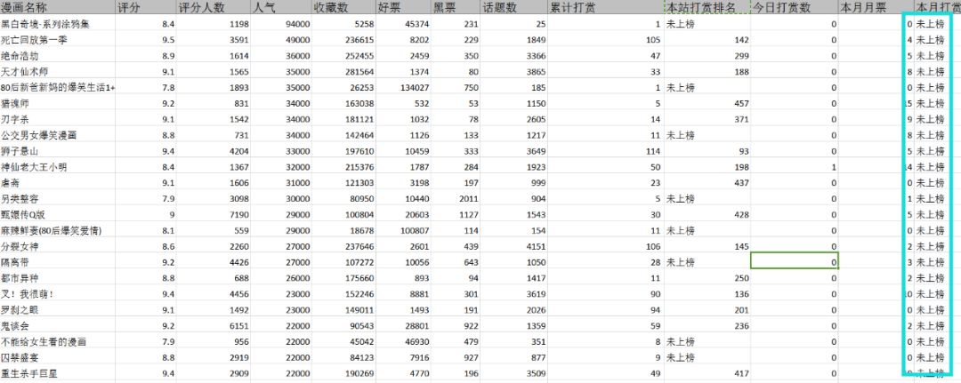
有些列的数据存在问题,不完整,而且部分字段数据不规范,需要从已有的样本数据中清除。
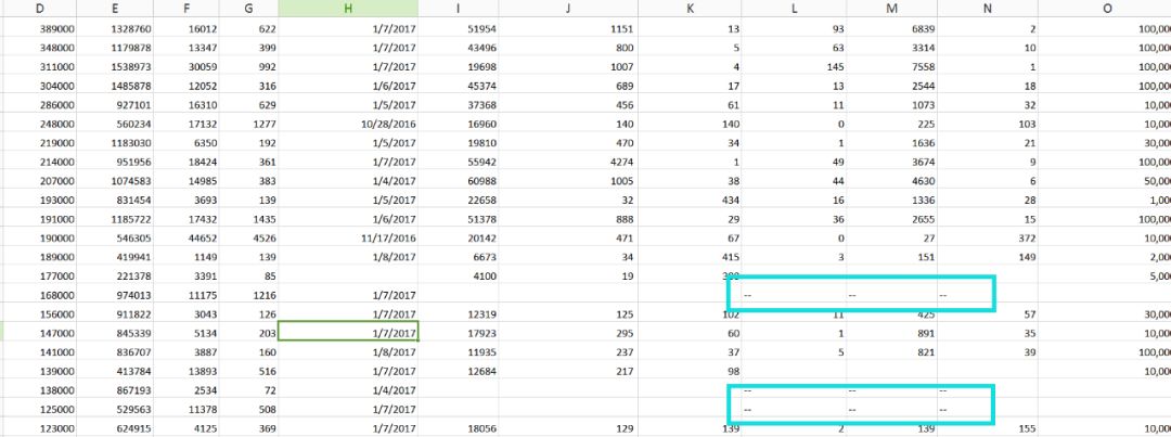
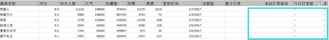
部分字段(如“本站打赏排名”和“本月打赏排名”)的数据值可以统一初始化,设置为0
整理后的有效数据为1707条,包含属性14个。
> dim(data1)
[1] 1707 14
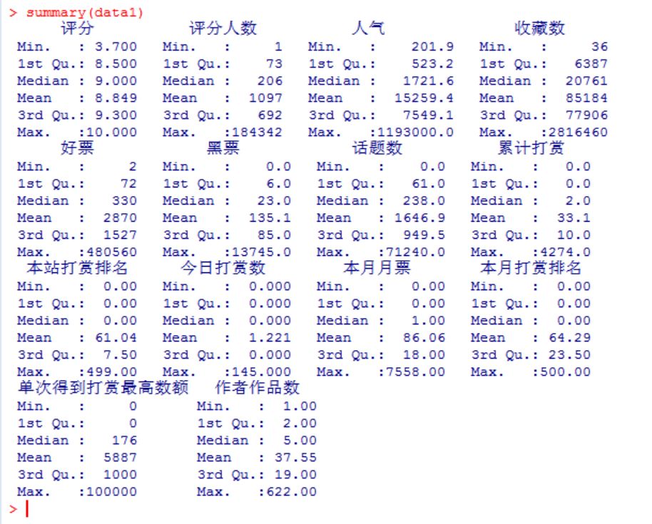
3.查看摘要信息
> head(data1)
评分 评分人数 人气 收藏数 好票 黑票 话题数 累计打赏 本站打赏排名
1 10.0 16310 1193000 726345 44198 2340 10597 1466 3
2 9.4 184342 964000 1429539 480560 13745 51279 2775 16
3 10.0 28730 836000 1307928 63000 2627 12600 392 56
4 9.6 54784 798000 2816460 74920 2092 51454 3594 6
5 9.4 59338 650000 1673324 165316 5030 61929 1817 30
6 9.6 52486 540000 1940672 78072 1919 67121 2751 10
今日打赏数 本月月票 本月打赏排名 单次得到打赏最高数额 作者作品数
1 0 0 0 5e+04 90
2 21 2582 16 1e+05 2
3 0 0 0 2e+04 90
4 79 6740 3 1e+05 3
5 27 3249 12 1e+05 1
6 83 5506 5 1e+05 39
There were 50 or more warnings (use warnings() to see the first 50)
> data1_cor <- cor(data1)
> head(cor(data1),5)
评分 评分人数 人气 收藏数 好票 黑票
评分 1.00000000 0.09356201 0.1389587 0.1840875 0.01174125 -0.02554861
评分人数 0.09356201 1.00000000 0.7034595 0.6423904 0.88315035 0.76918964
人气 0.13895874 0.70345953 1.0000000 0.7405844 0.56538974 0.53467002
收藏数 0.18408752 0.64239041 0.7405844 1.0000000 0.40939085 0.47503457
好票 0.01174125 0.88315035 0.5653897 0.4093909 1.00000000 0.73538951
话题数 累计打赏 本站打赏排名 今日打赏数 本月月票 本月打赏排名
评分 0.1431886 0.09704738 0.13391903 0.1036939 0.1083381 0.145318632
评分人数 0.6686533 0.72556029 0.03745862 0.4261345 0.5353641 0.008251173
人气 0.6806679 0.72023214 0.06655756 0.4499013 0.5371925 0.013771191
收藏数 0.8881343 0.73356768 0.18149364 0.6731396 0.7784286 0.133504827
好票 0.4490371 0.54607831 -0.02044299 0.2462322 0.3314277 -0.042333517
单次得到打赏最高数额 作者作品数
评分 0.1390566 -0.21872936
评分人数 0.3988320 -0.02447331
人气 0.3970846 -0.01516166
收藏数 0.5750740 -0.08028834
好票 0.2538240 -0.02903581
4.主成因子分析
library(psych)
data1_cor <- cor(data1)
确定因子数量
fa.parallel(data1_cor, n.obs = 112, fa = "both", n.iter = 100)
从碎石图可以看到:
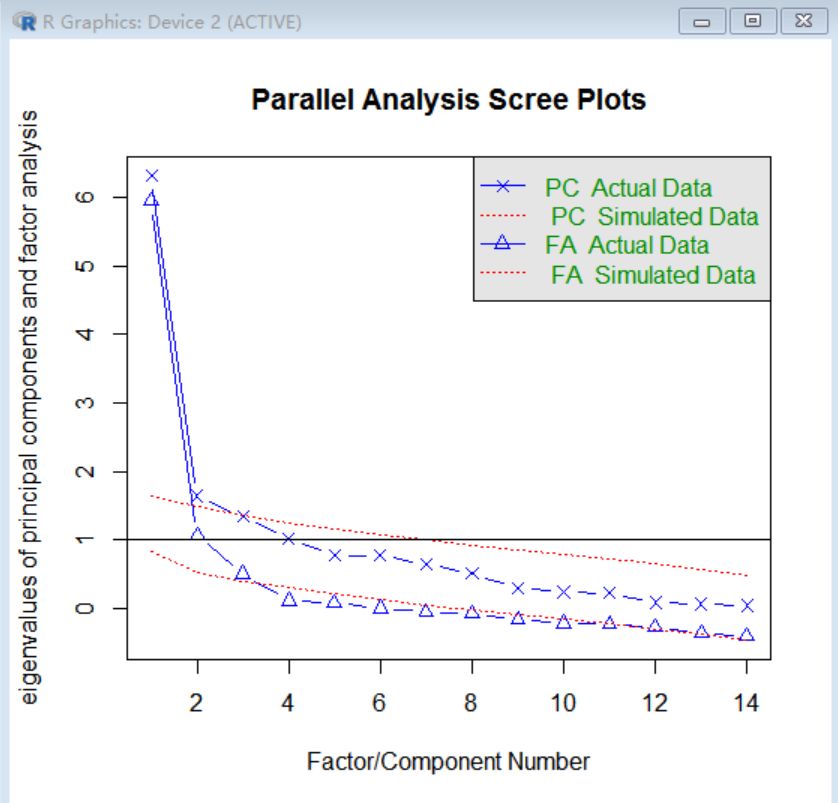
从这样的数据分析可以看到前3个会占据主要的部分,保留3个主成分即可。
接下来要做因子分析了,第一个参数是数据,第二个参数说明要保留三个主成分,第三个参数为旋转方法,为none,先不进行主成分旋转,第四个参数表示提取公因子的方法为最大似然法,不是机器学习的意思。
> fa_model1 <- fa(data1_cor, nfactors = 3, rotate = "none", fm = "ml")
输出的分析结果如下:
> fa_model1
Factor Analysis using method = ml
Call: fa(r = data1_cor, nfactors = 3, rotate = "none", fm = "ml")
Standardized loadings (pattern matrix) based upon correlation matrix
ML1 ML2 ML3 h2 u2 com
评分 0.12 0.03 0.19 0.0496 0.950 1.7
评分人数 0.61 0.76 -0.08 0.9573 0.043 1.9
人气 0.60 0.48 0.27 0.6645 0.336 2.4
收藏数 0.82 0.24 0.45 0.9344 0.066 1.7
好票 0.41 0.81 -0.26 0.8832 0.117 1.7
黑票 0.44 0.65 -0.10 0.6236 0.376 1.8
话题数 0.85 0.23 0.31 0.8648 0.135 1.4
累计打赏 0.76 0.35 0.11 0.7118 0.288 1.5
本站打赏排名 0.04 0.04 0.27 0.0741 0.926 1.1
今日打赏数 0.92 -0.18 -0.08 0.8778 0.122 1.1
本月月票 0.99 -0.10 -0.03 0.9950 0.005 1.0
本月打赏排名 0.00 0.03 0.25 0.0660 0.934 1.0
单次得到打赏最高数额 0.51 0.15 0.28 0.3566 0.643 1.7
作者作品数 -0.05 -0.01 -0.08 0.0084 0.992 1.6
ML1 ML2 ML3
SS loadings 5.15 2.18 0.73
Proportion Var 0.37 0.16 0.05
Cumulative Var 0.37 0.52 0.58
Proportion Explained 0.64 0.27 0.09
Cumulative Proportion 0.64 0.91 1.00
Mean item complexity = 1.6
Test of the hypothesis that 3 factors are sufficient.
The degrees of freedom for the null model are 91 and the objective function was 11.3
The degrees of freedom for the model are 52 and the objective function was 0.47
The root mean square of the residuals (RMSR) is 0.04
The df corrected root mean square of the residuals is 0.05
Fit based upon off diagonal values = 0.99
Measures of factor score adequacy
ML1 ML2 ML3
Correlation of (regression) scores with factors 1.00 0.98 0.92
Multiple R square of scores with factors 1.00 0.96 0.84
Minimum correlation of possible factor scores 0.99 0.92 0.69
为了减少误差,需要做因子旋转,这里使用的是正交旋转法,
fa_model2 <- fa(data1_cor, nfactors = 2, rotate = "varimax", fm = "ml")
> fa_model2
Factor Analysis using method = ml
Call: fa(r = data1_cor, nfactors = 3, rotate = "varimax", fm = "ml")
Standardized loadings (pattern matrix) based upon correlation matrix
ML2 ML1 ML3 h2 u2 com
评分 0.04 0.09 0.20 0.0496 0.950 1.4
评分人数 0.92 0.31 0.08 0.9573 0.043 1.2
人气 0.61 0.37 0.40 0.6645 0.336 2.5
收藏数 0.43 0.65 0.57 0.9344 0.066 2.7
好票 0.93 0.11 -0.10 0.8832 0.117 1.1
黑票 0.77 0.19 0.03 0.6236 0.376 1.1
话题数 0.45 0.69 0.43 0.8648 0.135 2.5
累计打赏 0.57 0.58 0.24 0.7118 0.288 2.3
本站打赏排名 0.01 0.01 0.27 0.0741 0.926 1.0
今日打赏数 0.16 0.92 0.00 0.8778 0.122 1.1
本月月票 0.25 0.96 0.07 0.9950 0.005 1.1
本月打赏排名 -0.01 -0.03 0.25 0.0660 0.934 1.0
单次得到打赏最高数额 0.26 0.40 0.35 0.3566 0.643 2.7
作者作品数 -0.01 -0.04 -0.08 0.0084 0.992 1.4
ML2 ML1 ML3
SS loadings 3.54 3.47 1.06
Proportion Var 0.25 0.25 0.08
Cumulative Var 0.25 0.50 0.58
Proportion Explained 0.44 0.43 0.13
Cumulative Proportion 0.44 0.87 1.00
Mean item complexity = 1.7
Test of the hypothesis that 3 factors are sufficient.
The degrees of freedom for the null model are 91 and the objective function was 11.3
The degrees of freedom for the model are 52 and the objective function was 0.47
The root mean square of the residuals (RMSR) is 0.04
The df corrected root mean square of the residuals is 0.05
Fit based upon off diagonal values = 0.99
Measures of factor score adequacy
ML2 ML1 ML3
Correlation of (regression) scores with factors 0.98 1.00 0.92
Multiple R square of scores with factors 0.96 0.99 0.85
Minimum correlation of possible factor scores 0.92 0.98 0.69
>
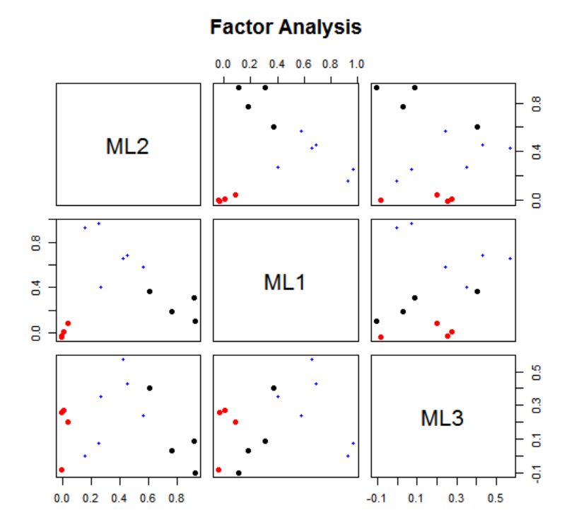
可以看到方差比例不变,但在各观测值上的载荷发生了改变
使用factor.plot函数对旋转结果进行可视化:
> factor.plot(fa_model2)
继续渲染,得到一个较为清晰的列表
> fa.diagram(fa_model2, simple = FALSE)
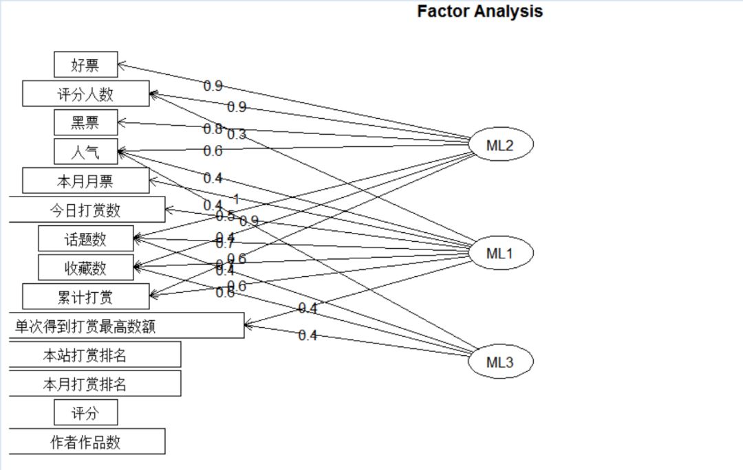
5.结论:
从以上数据可以看出,
第一主成分和“好票”,“评分人数”,“黑票”,“收藏数”相关性较高
第二主成分和“本月月票”,“今日打赏数”,“累计打赏”相关性较高
第三主成分和“人气”相关性较高。
相关链接:


 被折叠的 条评论
为什么被折叠?
被折叠的 条评论
为什么被折叠?
 到【灌水乐园】发言


