


1. Implied Volatility, 隐藏波动性
关于期权报价的分析?
Black-Scholes-Merton(1973) functions
#
#Valuation of European call options in Black-Scholes-Merton model
#incl. Vega function and implied volatility estimation
#bsm_functions.py
#

#Analytical Black-Scholes-Merton (BSM) Formula

def bsm_call_value(S0,K, T,r, sigma):
    """Valuation of European call option in BSM model.
    Analytical formula

    Parameters
    ==========
    S0 : float
         initial stok/index level
    K : float
        strike price
    T : float
        maturity date (in year fractions)
    r : float
        constant risk-free short rate
    sigma : float
        volatility factor in diffusion term


    Returns
    =======
    value : float
        present value of the European call option
        """

    from math import log, sqrt, exp
    from scipy import stats

    S0 = float(S0)
    d1 = (log(S0/K)+(r+0.5*sigma**2)*T)/(sigma*sqrt(T))
    d2 = (log(S0/K)+(r-0.5*sigma**2)*T)/(sigma*sqrt(T))
    value = (S0*stats.norm.cdf(d1,0.0,1.0)
            -K*exp(-r*T)*stats.norm.cdf(d2,0.0,1.0))
        #stats.norm.cdf --> cumulative distribution function 累计分布函数
        #                   for normal distribution

    return value

    #Vega function

    def bsm_vega(S0, K, T, r, sigma):
        '''Vega of European option in BSM model.

        Parameters
        ==========
        S0 : float
             initial stok/index level
        K : float
            strike price
        T : float
            maturity date (in year fractions)
        r : float
            constant risk-free short rate
        sigma : float
            volatility factor in diffusion term


        Returns
        =======
        vega : float
            partial derivative of BSM formula with respect to sigma, i.e. Vega
            '''
        from math import log, sqrt
        from scipy import stats

        S0 = float(S0)
        d1 = (log(S0/K)+(r+0.5*sigma**2)*T/(sigma*sqrt(T)))
        vega = S0*stats.norm.cdf(d1, 0.0, 1.0)*sqrt(T)


        #Implied volatility function
        def bsm_call_vol(S0, K, T, r, C0, sigma_est, it=100):
            '''Implied volatility of European call option in BSM model.

            Parameters
            ==========
            S0 : float
                 initial stok/index level
            K : float
                strike price
            T : float
                maturity date (in year fractions)
            r : float
                constant risk-free short rate
            sigma_est : float
                estimate of impl. volatility
            it : integer
                number of interations

            Returns
            =======
            sigma_est : float
                numericall estimated implied volatility

            '''

            for i in range(it):
                sigma_est -= ((bsm_call_value(S0, K, T, r, sigma_est)-C0)/bsm_vega(S0, K, T, r, sigma_est))
            return sigma_est
2. Monte Carlo simulation, 蒙特·卡罗方法(Monte Carlo method),也称统计模拟方法
跟股票指数有关?
Monte Carlo method是金融和数据科学的重要算法之一。可以解决高维度问题。
缺点,需要非常大的计算能力。
比较三种方法计算欧式期权(European Option)的Monte Carlo-based value
Pure Python : 用python的标准库计算Monte Carlo 值
Vectorized Numpy : 用Numpy库
Fully vertorized Numpy : 结合不同的数据公式来实现
Black-Scholes-Merton(1973) 随机微分方程
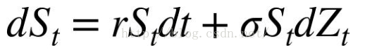
其中, Z是布朗运动系数(Brownian motion)
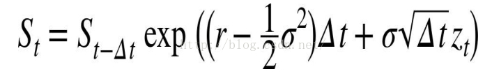
Euler discretization of SDE(stochastic differential equation)
使用Pure Python实现Monte Carlo valuation of European call option(欧式买方期权)
#
#Monte Carlo valuation of European call options with pure Python
#msc_pure_python.py
#

from time import time
from math import exp, sqrt, log
from random import gauss, seed

seed(20000)
t0=time()

#Parameters
S0=100 #initial value
K = 105. #strike price,成交价
T = 1.0 #maturity
r = 0.05 #riskless short rate
sigma = 0.2 #volatility
M = 50 #number of time steps
dt = T/M #length of time interval
I = 250000 #number of paths

# Simulating I paths with M time steps
S=[]
for i in range(I):
    path = []
    for t in range(M+1):
        if t==0:
            path.append(S0)
        else:
            z= gauss(0.0, 1.0)
            St = path[t-1]*exp((r-0.5*sigma**2)*dt
                                +sigma*sqrt(dt)*z)
            path.append(St)
    S.append(path)

#Calculating the Monte Carlo estimator
C0 = exp(-r*T)*sum([max(path[-1]-K,0) for path in S])/I

#Results output
tpy = time() - t0
print "European Option Value %7.3f"  %C0
print "Duration in Seconds   %7.3f" %tpy
输出结果:
European Option Value   7.999
Duration in Seconds    33.419
Monte Carlo valuation of European call option with Numpy(first version)
#
# Monte Carlo valuation of European call options with Numpy
# msc_vector_numpy.py
#

import math
import numpy as np
from time import time

np.random.seed(20000)
# 一般计算机的随机数都是伪随机数,以一个真随机数(种子)作为初始条件,然后用一定的算法不停迭代产生随机数
t0 = time()

#Parameters
S0 = 100.
K = 105.
T = 1.0
r = 0.05
sigma = 0.2
M = 50
dt = T/M
I = 250000

#Simulating I path with M time stemps
S = np.zeros((M+1, I))
S[0] = S0
for t in range(1, M+1):
    z = np.random.standard_normal(I) #pseudorandom numbers
    S[t] = S[t-1] * np.exp((r-0.5*sigma**2)*dt
                            +sigma*math.sqrt(dt)*z)
#vertorized operation per time step over all paths

# Calculating the Monte Carlo estimator
C0 = math.exp(-r*T)*np.sum(np.maximum(S[-1]-K, 0))/I

# Results output
tnp1 = time() - t0
print "European Option Value %7.3f"%C0
print "Duration in Seconds   %7.3f"%tnp1
输出结果
European Option Value   8.037
Duration in Seconds     1.382
Full Vetorization wtih Log Euler Scheme
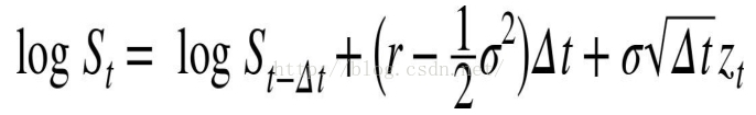
采用Log微分,Euler discretization of SDE(log verion)
#
# Monte Carlo valuation of European call options with Numpy (log version)
# msc_full_vector_numpy.py
#

import math
from numpy import *
from time import time


random.seed(20000)
t0 = time()

#Parameters
S0 = 100.
K = 105.
T = 1.0
r = 0.05
sigma = 0.2
M = 50
dt = T/M
I = 250000

#Simulating I paths with M time steps
S = S0*exp(cumsum((r-0.5*sigma**2)*dt+sigma*math.sqrt(dt)*random.standard_normal((M+1, I)),axis=0))
#sum instead of cumsum would also do if only the final values are of interest
S[0] = S0
C0 = math.exp(-r*T)*sum(maximum(S[-1]-K,0))/I

# Results output
tnp1 = time() - t0
print "European Option Value %7.3f"%C0
print "Duration in Seconds   %7.3f"%tnp1
输出结果:
European Option Value 8.166
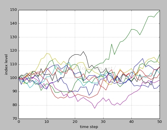
Duration in Seconds 2.020图形化模拟过程
import matplotlib.pyplot as plt
plt.plot(S[:, :10])
plt.grid(True)
plt.xlabel('time step')
plt.ylabel('index level')
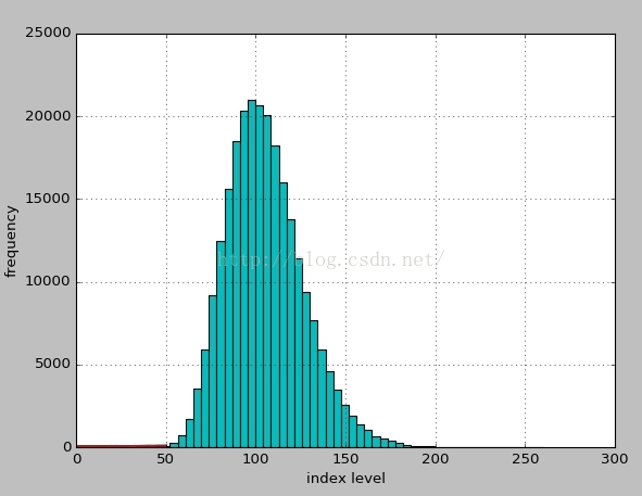
显示模拟指数的频率
plt.hist(S[-1], bins = 50)
plt.grid(True)
plt.xlabel('index level')
plt.ylabel('frequency')
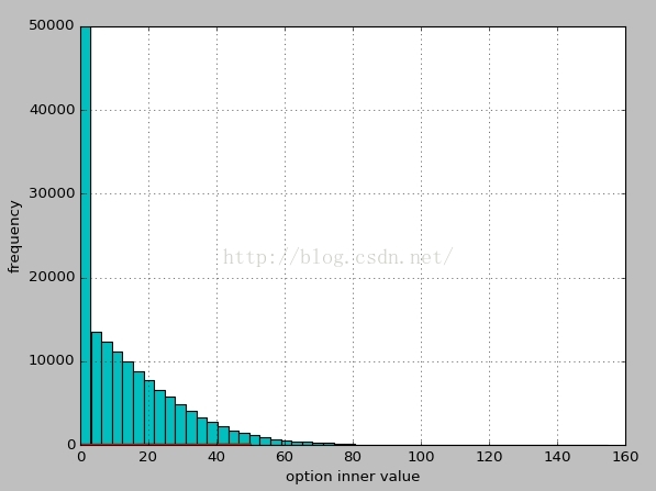
option inner value??
plt.hist(np.maximum(S[-1]-K,0), bins = 50)
plt.grid(True)
plt.xlabel('option inner value')
plt.ylabel('frequency')
plt.ylim(0,50000)
3. Technical Analysis, 技术分析
根据历史数据回测投资策略的趋势信号
从yahoo finance下载SP500指数数据,并画出42日均线和252日均线
import numpy as np
import pandas as pd
import pandas.io.data as web


sp500 = web.DataReader('^GSPC',data_source='yahoo', start = '1/1/2000', end = '4/14/2014')
#print sp500.info()


#42天均线,和252天均线
sp500['42d'] = np.round(pd.rolling_mean(sp500['Close'],window=42),2)
sp500['252d'] = np.round(pd.rolling_mean(sp500['Close'],window=252),2)

sp500[['Close','42d','252d']].plot(grid = True, figsize = (8,5))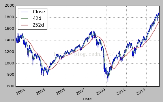


 1089
1089

 被折叠的 条评论
为什么被折叠?
被折叠的 条评论
为什么被折叠?
 到【灌水乐园】发言


