


目录
【思考题】对比3.1基于Logistic回归的二分类任务和 4.2 基于前馈神经网络的二分类任务谈谈自己的看法
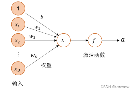
4.1 神经元
4.1.1 净活性值
使用pytorch计算一组输入的净活性值z
净活性值z经过一个非线性函数f(·)后,得到神经元的活性值a
使用pytorch计算一组输入的净活性值,代码实现如下:
import torch

# 2个特征数为5的样本
X = torch.rand(size=[2, 5])

# 含有5个参数的权重向量
w = torch.rand(size=[5, 1])
# 偏置项
b = torch.rand(size=[1, 1])

# 使用'torch.matmul'实现矩阵相乘
z = torch.matmul(X, w) + b
print("input X:", X)
print("weight w:", w, "\nbias b:", b)
print("output z:", z)
结果如下:
input X: tensor([[0.0473, 0.5967, 0.1484, 0.2198, 0.8467],
        [0.3004, 0.2063, 0.2169, 0.0047, 0.5351]])
weight w: Parameter containing:
tensor([[ 0.4313, -0.0266, -0.0397,  0.1398, -0.3974]], requires_grad=True)
bias b: tensor([[0.2483]])
output z: tensor([[-0.0588],
        [ 0.1518]], grad_fn=<AddBackward0>)
也可以使用相应函数torch.nn.Linear(features_in, features_out, bias=False)完成上述转换:
import torch

# 2个特征数为5的样本
X = torch.rand(size=[2, 5])

# 含有5个参数的权重向量
fc = torch.nn.Linear(5, 1, True)
# 偏置项
b = torch.rand(size=[1, 1])

# 使用'torch.matmul'实现矩阵相乘
z = fc(X) + b
print("input X:", X)
print("weight w:", fc.weight, "\nbias b:", b)
print("output z:", z)
结果如下:
input X: tensor([[0.0473, 0.5967, 0.1484, 0.2198, 0.8467],
        [0.3004, 0.2063, 0.2169, 0.0047, 0.5351]])
weight w: Parameter containing:
tensor([[ 0.4313, -0.0266, -0.0397,  0.1398, -0.3974]], requires_grad=True)
bias b: tensor([[0.2483]])
output z: tensor([[-0.0588],
[ 0.1518]], grad_fn=<AddBackward0>)【思考题】加权相加与仿射变换之间有什么区别和联系?
加权相加:输入向量乘对应权重
再相加,即
仿射变换是指在几何中,一个向量空间进行一次线性变换并接上一个平移,变换为另一个向量空间。一个对向量平移
,与旋转放大缩小
的仿射映射为
区别:几何意义上,相权相加是一种线性变换,变换前后位置不发生变化,仿射变换会发生平移等操作,位置发生了改变
联系:仿射变换中,当位移量b等于0时,就是线性变换
4.1.2 激活函数
激活函数通常为非线性函数,可以增强神经网络的表示能力和学习能力。
常用的激活函数有S型函数和ReLU函数。
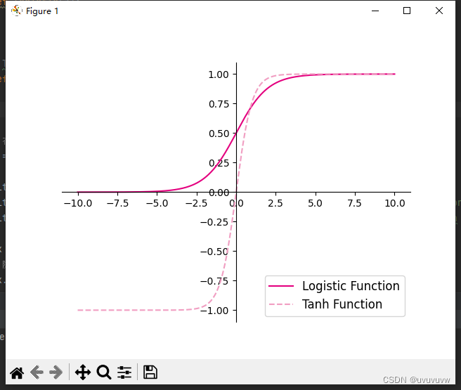
4.1.2.1 Sigmoid 型函数
常用的 Sigmoid 型函数有 Logistic 函数和 Tanh 函数。
- 使用python实现并可视化“Logistic函数、Tanh函数”
import matplotlib.pyplot as plt
import torch

# Logistic函数
def logistic(z):
    return 1.0 / (1.0 + torch.exp(-z))


# Tanh函数
def tanh(z):
    return (torch.exp(z) - torch.exp(-z)) / (torch.exp(z) + torch.exp(-z))


# 在[-10,10]的范围内生成10000个输入值,用于绘制函数曲线
z = torch.linspace(-10, 10, 10000)

plt.figure()
plt.plot(z.tolist(), logistic(z).tolist(), color='#e4007f', label="Logistic Function")
plt.plot(z.tolist(), tanh(z).tolist(), color='#f19ec2', linestyle='--', label="Tanh Function")

ax = plt.gca()  # 获取轴,默认有4个
# 隐藏两个轴,通过把颜色设置成none
ax.spines['top'].set_color('none')
ax.spines['right'].set_color('none')
# 调整坐标轴位置
ax.spines['left'].set_position(('data', 0))
ax.spines['bottom'].set_position(('data', 0))
plt.legend(loc='lower right', fontsize='large')

plt.savefig('fw-logistic-tanh.pdf')
plt.show()
可视化结果如图:
- 在飞桨中,可以通过调用
paddle.nn.functional.sigmoid和paddle.nn.functional.tanh实现对张量的Logistic和Tanh计算。在pytorch中找到相应函数并测试。import matplotlib.pyplot as plt import torch # 在[-10,10]的范围内生成10000个输入值,用于绘制函数曲线 z = torch.linspace(-10, 10, 10000) plt.figure() plt.plot(z.tolist(), torch.sigmoid(z).tolist(), color='#e4007f', label="Logistic Function") plt.plot(z.tolist(), torch.tanh(z).tolist(), color='#f19ec2', linestyle='--', label="Tanh Function") ax = plt.gca() # 获取轴,默认有4个 # 隐藏两个轴,通过把颜色设置成none ax.spines['top'].set_color('none') ax.spines['right'].set_color('none') # 调整坐标轴位置 ax.spines['left'].set_position(('data', 0)) ax.spines['bottom'].set_position(('data', 0)) plt.legend(loc='lower right', fontsize='large') plt.savefig('fw-logistic-tanh.pdf') plt.show()pytorch中用torch.sigmoid()和torch.tanh()函数也可以实现上述功能。结果与1相同。
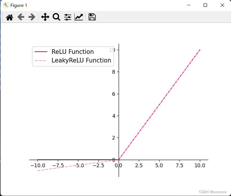
4.1.2.2 ReLU型函数
常见的ReLU函数有ReLU和带泄露的ReLU(Leaky ReLU)
- 使用python实现并可视化可视化“ReLU、带泄露的ReLU的函数”
import torch
import matplotlib.pyplot as plt


# ReLU
def relu(z):
    return torch.maximum(z, torch.tensor(0.))


# 带泄露的ReLU
def leaky_relu(z, negative_slope=0.1):
    a1 = ((z > 0).to(torch.float32) * z)
    a2 = (z <= 0).to(torch.float32) * (negative_slope * z)
    return a1 + a2


# 在[-10,10]的范围内生成一系列的输入值,用于绘制relu、leaky_relu的函数曲线
z = torch.linspace(-10, 10, 10000)

plt.figure()
plt.plot(z.tolist(), relu(z).tolist(), color="#e4007f", label="ReLU Function")
plt.plot(z.tolist(), leaky_relu(z).tolist(), color="#f19ec2", linestyle="--", label="LeakyReLU Function")

ax = plt.gca()
ax.spines['top'].set_color('none')
ax.spines['right'].set_color('none')
ax.spines['left'].set_position(('data', 0))
ax.spines['bottom'].set_position(('data', 0))
plt.legend(loc='upper left', fontsize='large')
plt.savefig('fw-relu-leakyrelu.pdf')
plt.show()
可视化结果如图:
4.2 基于前馈神经网络的二分类任务
4.2.1 数据集构建
使用第3.1.1节中构建的二分类数据集:Moon1000数据集,其中训练集640条、验证集160条、测试集200条。该数据集的数据是从两个带噪音的弯月形状数据分布中采样得到,每个样本包含2个特征。
数据集构建函数:
import math
import torch


# 新增make_moons函数
def make_moons(n_samples, shuffle, noise):
    """
    生成带噪音的弯月形状数据
    输入:
        - n_samples:数据量大小,数据类型为int
        - shuffle:是否打乱数据,数据类型为bool
        - noise:以多大的程度增加噪声,数据类型为None或float,noise为None时表示不增加噪声
    输出:
        - X:特征数据,shape=[n_samples,2]
        - y:标签数据, shape=[n_samples]
    """
    n_samples_out = n_samples // 2
    n_samples_in = n_samples - n_samples_out

    # 采集第1类数据,特征为(x,y)
    # 使用'torch.linspace'在0到pi上均匀取n_samples_out个值
    # 使用'torch.cos'计算上述取值的余弦值作为特征1,使用'torch.sin'计算上述取值的正弦值作为特征2
    outer_circ_x = torch.cos(torch.linspace(0, math.pi, n_samples_out))
    outer_circ_y = torch.sin(torch.linspace(0, math.pi, n_samples_out))

    inner_circ_x = 1 - torch.cos(torch.linspace(0, math.pi, n_samples_in))
    inner_circ_y = 0.5 - torch.sin(torch.linspace(0, math.pi, n_samples_in))

    print('outer_circ_x.shape:', outer_circ_x.shape, 'outer_circ_y.shape:', outer_circ_y.shape)
    print('inner_circ_x.shape:', inner_circ_x.shape, 'inner_circ_y.shape:', inner_circ_y.shape)

    # 使用'torch.concat'将两类数据的特征1和特征2分别延维度0拼接在一起,得到全部特征1和特征2
    # 使用'torch.stack'将两类特征延维度1堆叠在一起
    X = torch.stack(
        [torch.concat([outer_circ_x, inner_circ_x]),
         torch.concat([outer_circ_y, inner_circ_y])],
        dim=1
    )

    print('after concat shape:', torch.concat([outer_circ_x, inner_circ_x]).shape)
    print('X shape:', X.shape)

    # 使用'torch. zeros'将第一类数据的标签全部设置为0
    # 使用'torch. ones'将第一类数据的标签全部设置为1
    y = torch.concat(
        [torch.zeros([n_samples_out]), torch.ones([n_samples_in])]
    )

    print('y shape:', y.shape)

    # 如果shuffle为True,将所有数据打乱
    if shuffle:
        # 使用'torch.randperm'生成一个数值在0到X.shape[0],随机排列的一维Tensor做索引值,用于打乱数据
        idx = torch.randperm(X.shape[0])
        X = X[idx]
        y = y[idx]

    # 如果noise不为None,则给特征值加入噪声
    if noise is not None:
        # 使用'torch.normal'生成符合正态分布的随机Tensor作为噪声,并加到原始特征上
        X += torch.normal(mean=0.0, std=noise, size=X.shape)

    return X, y
数据集采样:
from nndl.dataset import make_moons

# 采样1000个样本
n_samples = 1000
X, y = make_moons(n_samples=n_samples, shuffle=True, noise=0.2)

num_train = 640
num_dev = 160
num_test = 200

X_train, y_train = X[:num_train], y[:num_train]
X_dev, y_dev = X[num_train:num_train + num_dev], y[num_train:num_train + num_dev]
X_test, y_test = X[num_train + num_dev:], y[num_train + num_dev:]

y_train = y_train.reshape([-1,1])
y_dev = y_dev.reshape([-1,1])
y_test = y_test.reshape([-1,1])
最终构建的数据集结果:
outer_circ_x.shape: torch.Size([500]) outer_circ_y.shape: torch.Size([500])
inner_circ_x.shape: torch.Size([500]) inner_circ_y.shape: torch.Size([500])
after concat shape: torch.Size([1000])
X shape: torch.Size([1000, 2])
y shape: torch.Size([1000])
4.2.2 模型构建
为了更高效的构建前馈神经网络,我们先定义每一层的算子,然后再通过算子组合构建整个前馈神经网络。
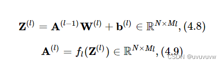
4.2.2.1 线性层算子
公式(4.8)对应一个线性层算子,权重参数采用默认的随机初始化,偏置采用默认的零初始化。代码实现如下:
from nndl.dataset import make_moons
from nndl.op import Op
import torch


class Linear(Op):
    def __init__(self, input_size, output_size, name, weight_init=torch.randn, bias_init=torch.zeros):
        """
        输入:
            - input_size:输入数据维度
            - output_size:输出数据维度
            - name:算子名称
            - weight_init:权重初始化方式,默认使用'paddle.standard_normal'进行标准正态分布初始化
            - bias_init:偏置初始化方式,默认使用全0初始化
        """

        self.params = {}
        # 初始化权重
        self.params['W'] = weight_init([input_size, output_size])
        # 初始化偏置
        self.params['b'] = bias_init([1, output_size])
        self.inputs = None

        self.name = name

    def forward(self, inputs):
        """
        输入:
            - inputs:shape=[N,input_size], N是样本数量
        输出:
            - outputs:预测值,shape=[N,output_size]
        """
        self.inputs = inputs

        outputs = torch.matmul(self.inputs, self.params['W']) + self.params['b']
        return outputs
4.2.2.2 Logistic算子(激活函数)
class Logistic(Op):
    def __init__(self):
        self.inputs = None
        self.outputs = None

    def forward(self, inputs):
        """
        输入:
            - inputs: shape=[N,D]
        输出:
            - outputs:shape=[N,D]
        """
        outputs = 1.0 / (1.0 + torch.exp(-inputs))
        self.outputs = outputs
        return outputs
4.2.2.3 层的串行组合
实现一个两层的用于二分类任务的前馈神经网络,选用Logistic作为激活函数,可以利用上面实现的线性层和激活函数算子来组装,代码实现如下:
class Model_MLP_L2(Op):
    def __init__(self, input_size, hidden_size, output_size):
        """
        输入:
            - input_size:输入维度
            - hidden_size:隐藏层神经元数量
            - output_size:输出维度
        """
        super().__init__()
        self.fc1 = Linear(input_size, hidden_size, name="fc1")
        self.act_fn1 = Logistic()
        self.fc2 = Linear(hidden_size, output_size, name="fc2")
        self.act_fn2 = Logistic()

    def __call__(self, X):
        return self.forward(X)

    def forward(self, X):
        """
        输入:
            - X:shape=[N,input_size], N是样本数量
        输出:
            - a2:预测值,shape=[N,output_size]
        """
        z1 = self.fc1(X)
        a1 = self.act_fn1(z1)
        z2 = self.fc2(a1)
        a2 = self.act_fn2(z2)
        return a2
实例化一个两层的前馈网络,令其输入层维度为5,隐藏层维度为10,输出层维度为1。
并随机生成一条长度为5的数据输入两层神经网络,观察输出结果,测试代码如下:
# 实例化模型
model = Model_MLP_L2(input_size=5, hidden_size=10, output_size=1)
# 随机生成1条长度为5的数据
X = torch.rand(size=[1, 5])
result = model(X)
print("result: ", result)
测试结果如下:
result: tensor([[0.9688]])4.2.3 损失函数
二分类交叉熵损失函数: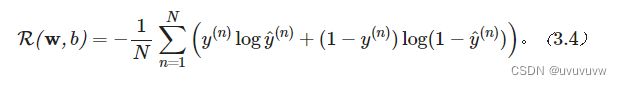
代码实现如下:
class BinaryCrossEntropyLoss(op.Op):
    def __init__(self):
        self.predicts = None
        self.labels = None
        self.num = None

    def __call__(self, predicts, labels):
        return self.forward(predicts, labels)

    def forward(self, predicts, labels):
        """
        输入:
            - predicts:预测值,shape=[N, 1],N为样本数量
            - labels:真实标签,shape=[N, 1]
        输出:
            - 损失值:shape=[1]
        """
        self.predicts = predicts
        self.labels = labels
        self.num = self.predicts.shape[0]
        loss = -1. / self.num * (torch.matmul(self.labels.t(), torch.log(self.predicts)) + torch.matmul((1-self.labels.t()), torch.log(1-self.predicts)))
        loss = torch.squeeze(loss, 1)
        return loss
4.2.4 模型优化
神经网络的层数通常比较深,其梯度计算和上一章中的线性分类模型的不同的点在于:
线性模型通常比较简单可以直接计算梯度,而神经网络相当于一个复合函数,需要利用链式法则进行反向传播来计算梯度。
4.2.4.1 反向传播算法
- 前馈计算每一层的净活性值
和激活值
,直到最后一层;
- 反向传播计算每一层的误差项
- 计算每一层参数的梯度,并更新参数。
在模型训练过程中,我们首先执行模型的forward(),再执行模型的backward(),就得到了所有参数的梯度,之后再利用优化器迭代更新参数。
以这我们这节中构建的两层全连接前馈神经网络Model_MLP_L2为例,下图给出了其前向和反向计算过程:
下面我们按照反向的梯度传播顺序,为每个算子添加backward()方法,并在其中实现每一层参数的梯度的计算。
4.2.4.2 损失函数
二分类交叉熵损失函数对神经网络的输出 的偏导数为:
实现损失函数的backward(),代码实现如下:
# 实现交叉熵损失函数
class BinaryCrossEntropyLoss(Op):
    def __init__(self, model):
        super().__init__()
        self.predicts = None
        self.labels = None
        self.num = None

        self.model = model

    def __call__(self, predicts, labels):
        return self.forward(predicts, labels)

    def forward(self, predicts, labels):
        """
        输入:
            - predicts:预测值,shape=[N, 1],N为样本数量
            - labels:真实标签,shape=[N, 1]
        输出:
            - 损失值:shape=[1]
        """
        self.predicts = predicts
        self.labels = labels
        self.num = self.predicts.shape[0]
        loss = -1. / self.num * (torch.matmul(self.labels.t(), torch.log(self.predicts))
                                 + torch.matmul((1 - self.labels.t()), torch.log(1 - self.predicts)))

        loss = torch.squeeze(loss, 1)
        return loss

    def backward(self):
        # 计算损失函数对模型预测的导数
        loss_grad_predicts = -1.0 * (self.labels / self.predicts -
                                     (1 - self.labels) / (1 - self.predicts)) / self.num

        # 梯度反向传播
        self.model.backward(loss_grad_predicts)
4.2.4.3 Logistic算子
由于Logistic函数中没有参数,这里不需要在backward()方法中计算该算子参数的梯度。
class Logistic(Op):
    def __init__(self):
        self.inputs = None
        self.outputs = None
        self.params = None

    def forward(self, inputs):
        outputs = 1.0 / (1.0 + torch.exp(-inputs))
        self.outputs = outputs
        return outputs

    def backward(self, grads):
        # 计算Logistic激活函数对输入的导数
        outputs_grad_inputs = torch.multiply(self.outputs, (1.0 - self.outputs))
        return torch.multiply(grads, outputs_grad_inputs)
4.2.4.4 线性层
线性层输入的梯度
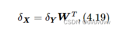
计算线性层参数的梯度
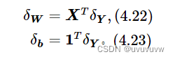
具体实现代码如下:
class Linear(Op):
    def __init__(self, input_size, output_size, name, weight_init=torch.randn, bias_init=torch.zeros):
        super().__init__()
        self.params = {}
        self.params['W'] = weight_init([input_size, output_size])
        self.params['b'] = bias_init([1, output_size])
        self.inputs = None
        self.grads = {}
        self.name = name

    def forward(self, inputs):
        self.inputs = inputs
        outputs = torch.matmul(self.inputs, self.params['W']) + self.params['b']
        return outputs

    def backward(self, grads):
        """
        输入:
            - grads:损失函数对当前层输出的导数
        输出:
            - 损失函数对当前层输入的导数
        """
        self.grads['W'] = torch.matmul(self.inputs.T, grads)
        self.grads['b'] = torch.sum(grads, 0)

        # 线性层输入的梯度
        return torch.matmul(grads, self.params['W'].T)
4.2.4.5 整个网络
实现完整的两层神经网络的前向和反向计算。代码实现如下:
class Model_MLP_L2(Op):
    def __init__(self, input_size, hidden_size, output_size):
        # 线性层
        super().__init__()
        self.fc1 = Linear(input_size, hidden_size, name="fc1")
        # Logistic激活函数层
        self.act_fn1 = Logistic()
        self.fc2 = Linear(hidden_size, output_size, name="fc2")
        self.act_fn2 = Logistic()

        self.layers = [self.fc1, self.act_fn1, self.fc2, self.act_fn2]

    def __call__(self, X):
        return self.forward(X)

    # 前向计算
    def forward(self, X):
        z1 = self.fc1(X)
        a1 = self.act_fn1(z1)
        z2 = self.fc2(a1)
        a2 = self.act_fn2(z2)
        return a2

    # 反向计算
    def backward(self, loss_grad_a2):
        loss_grad_z2 = self.act_fn2.backward(loss_grad_a2)
        loss_grad_a1 = self.fc2.backward(loss_grad_z2)
        loss_grad_z1 = self.act_fn1.backward(loss_grad_a1)
        loss_grad_inputs = self.fc1.backward(loss_grad_z1)
4.2.4.6 优化器
在计算好神经网络参数的梯度之后,我们将梯度下降法中参数的更新过程实现在优化器中。
与第3章中实现的梯度下降优化器SimpleBatchGD不同的是,此处的优化器需要遍历每层,对每层的参数分别做更新。
from nndl.opitimizer import Optimizer

class BatchGD(Optimizer):
    def __init__(self, init_lr, model):
        super(BatchGD, self).__init__(init_lr=init_lr, model=model)

    def step(self):
        # 参数更新
        for layer in self.model.layers:  # 遍历所有层
            if isinstance(layer.params, dict):
                for key in layer.params.keys():
                    layer.params[key] = layer.params[key] - self.init_lr * layer.grads[key]
4.2.5 完善Runner类:RunnerV2_1
基于3.1.6实现的 RunnerV2 类主要针对比较简单的模型。而在本章中,模型由多个算子组合而成,通常比较复杂,因此本节继续完善并实现一个改进版: RunnerV2_1类,其主要加入的功能有:
- 支持自定义算子的梯度计算,在训练过程中调用
self.loss_fn.backward()从损失函数开始反向计算梯度; - 每层的模型保存和加载,将每一层的参数分别进行保存和加载。
import os


class RunnerV2_1(object):
    def __init__(self, model, optimizer, metric, loss_fn, **kwargs):
        self.model = model
        self.optimizer = optimizer
        self.loss_fn = loss_fn
        self.metric = metric

        # 记录训练过程中的评估指标变化情况
        self.train_scores = []
        self.dev_scores = []

        # 记录训练过程中的评价指标变化情况
        self.train_loss = []
        self.dev_loss = []

    def train(self, train_set, dev_set, **kwargs):
        # 传入训练轮数,如果没有传入值则默认为0
        num_epochs = kwargs.get("num_epochs", 0)
        # 传入log打印频率,如果没有传入值则默认为100
        log_epochs = kwargs.get("log_epochs", 100)

        # 传入模型保存路径
        save_dir = kwargs.get("save_dir", None)

        # 记录全局最优指标
        best_score = 0
        # 进行num_epochs轮训练
        for epoch in range(num_epochs):
            X, y = train_set
            # 获取模型预测
            logits = self.model(X)
            # 计算交叉熵损失
            trn_loss = self.loss_fn(logits, y)  # return a tensor

            self.train_loss.append(trn_loss.item())
            # 计算评估指标
            trn_score = self.metric(logits, y).item()
            self.train_scores.append(trn_score)

            self.loss_fn.backward()

            # 参数更新
            self.optimizer.step()

            dev_score, dev_loss = self.evaluate(dev_set)
            # 如果当前指标为最优指标,保存该模型
            if dev_score > best_score:
                print(f"[Evaluate] best accuracy performence has been updated: {best_score:.5f} --> {dev_score:.5f}")
                best_score = dev_score
                if save_dir:
                    self.save_model(save_dir)

            if log_epochs and epoch % log_epochs == 0:
                print(f"[Train] epoch: {epoch}/{num_epochs}, loss: {trn_loss.item()}")

    def evaluate(self, data_set):
        X, y = data_set
        # 计算模型输出
        logits = self.model(X)
        # 计算损失函数
        loss = self.loss_fn(logits, y).item()
        self.dev_loss.append(loss)
        # 计算评估指标
        score = self.metric(logits, y).item()
        self.dev_scores.append(score)
        return score, loss

    def predict(self, X):
        return self.model(X)

    def save_model(self, save_dir):
        # 对模型每层参数分别进行保存,保存文件名称与该层名称相同
        for layer in self.model.layers:  # 遍历所有层
            if isinstance(layer.params, dict):
                torch.save(layer.params, os.path.join(save_dir, layer.name + ".pdparams"))

    def load_model(self, model_dir):
        # 获取所有层参数名称和保存路径之间的对应关系
        model_file_names = os.listdir(model_dir)
        name_file_dict = {}
        for file_name in model_file_names:
            name = file_name.replace(".pdparams", "")
            name_file_dict[name] = os.path.join(model_dir, file_name)

        # 加载每层参数
        for layer in self.model.layers:  # 遍历所有层
            if isinstance(layer.params, dict):
                name = layer.name
                file_path = name_file_dict[name]
                layer.params = torch.load(file_path)
4.2.6 模型训练
基于RunnerV2_1,使用训练集和验证集进行模型训练,共训练2000个epoch。评价指标为第章介绍的accuracy。代码实现如下:
from nndl.metric import accuracy

torch.manual_seed(102)
epoch_num = 1000

model_saved_dir = "model"

# 输入层维度为2
input_size = 2
# 隐藏层维度为5
hidden_size = 5
# 输出层维度为1
output_size = 1

# 定义网络
model = Model_MLP_L2(input_size=input_size, hidden_size=hidden_size, output_size=output_size)

# 损失函数
loss_fn = BinaryCrossEntropyLoss(model)

# 优化器
learning_rate = 0.2
optimizer = BatchGD(learning_rate, model)

# 评价方法
metric = accuracy

# 实例化RunnerV2_1类,并传入训练配置
runner = RunnerV2_1(model, optimizer, metric, loss_fn)

runner.train([X_train, y_train], [X_dev, y_dev], num_epochs=epoch_num, log_epochs=50, save_dir=model_saved_dir)
结果如下:
[Evaluate] best accuracy performence has been updated: 0.00000 --> 0.30625
[Train] epoch: 0/1000, loss: 0.8921629190444946
[Evaluate] best accuracy performence has been updated: 0.30625 --> 0.32500
[Evaluate] best accuracy performence has been updated: 0.32500 --> 0.33125
[Evaluate] best accuracy performence has been updated: 0.33125 --> 0.34375
[Evaluate] best accuracy performence has been updated: 0.34375 --> 0.35000
[Evaluate] best accuracy performence has been updated: 0.35000 --> 0.37500
[Evaluate] best accuracy performence has been updated: 0.37500 --> 0.40625
[Evaluate] best accuracy performence has been updated: 0.40625 --> 0.43125
[Evaluate] best accuracy performence has been updated: 0.43125 --> 0.46250
[Evaluate] best accuracy performence has been updated: 0.46250 --> 0.46875
[Evaluate] best accuracy performence has been updated: 0.46875 --> 0.47500
[Evaluate] best accuracy performence has been updated: 0.47500 --> 0.50000
[Evaluate] best accuracy performence has been updated: 0.50000 --> 0.51875
[Evaluate] best accuracy performence has been updated: 0.51875 --> 0.55625
[Evaluate] best accuracy performence has been updated: 0.55625 --> 0.56875
[Evaluate] best accuracy performence has been updated: 0.56875 --> 0.58750
[Evaluate] best accuracy performence has been updated: 0.58750 --> 0.60625
[Evaluate] best accuracy performence has been updated: 0.60625 --> 0.62500
[Evaluate] best accuracy performence has been updated: 0.62500 --> 0.64375
[Evaluate] best accuracy performence has been updated: 0.64375 --> 0.66250
[Evaluate] best accuracy performence has been updated: 0.66250 --> 0.67500
[Evaluate] best accuracy performence has been updated: 0.67500 --> 0.68125
[Evaluate] best accuracy performence has been updated: 0.68125 --> 0.68750
[Evaluate] best accuracy performence has been updated: 0.68750 --> 0.70625
[Evaluate] best accuracy performence has been updated: 0.70625 --> 0.71250
[Evaluate] best accuracy performence has been updated: 0.71250 --> 0.72500
[Evaluate] best accuracy performence has been updated: 0.72500 --> 0.73125
[Evaluate] best accuracy performence has been updated: 0.73125 --> 0.73750
[Evaluate] best accuracy performence has been updated: 0.73750 --> 0.74375
[Evaluate] best accuracy performence has been updated: 0.74375 --> 0.75000
[Train] epoch: 50/1000, loss: 0.5253771543502808
[Evaluate] best accuracy performence has been updated: 0.75000 --> 0.76250
[Evaluate] best accuracy performence has been updated: 0.76250 --> 0.76875
[Evaluate] best accuracy performence has been updated: 0.76875 --> 0.77500
[Evaluate] best accuracy performence has been updated: 0.77500 --> 0.78125
[Evaluate] best accuracy performence has been updated: 0.78125 --> 0.78750
[Evaluate] best accuracy performence has been updated: 0.78750 --> 0.79375
[Train] epoch: 100/1000, loss: 0.41670581698417664
[Evaluate] best accuracy performence has been updated: 0.79375 --> 0.80000
[Evaluate] best accuracy performence has been updated: 0.80000 --> 0.80625
[Train] epoch: 150/1000, loss: 0.3654296100139618
[Evaluate] best accuracy performence has been updated: 0.80625 --> 0.81250
[Evaluate] best accuracy performence has been updated: 0.81250 --> 0.81875
[Evaluate] best accuracy performence has been updated: 0.81875 --> 0.82500
[Evaluate] best accuracy performence has been updated: 0.82500 --> 0.83125
[Evaluate] best accuracy performence has been updated: 0.83125 --> 0.83750
[Train] epoch: 200/1000, loss: 0.3365909159183502
[Evaluate] best accuracy performence has been updated: 0.83750 --> 0.84375
[Train] epoch: 250/1000, loss: 0.31878677010536194
[Train] epoch: 300/1000, loss: 0.3072616755962372
[Train] epoch: 350/1000, loss: 0.2996121942996979
[Train] epoch: 400/1000, loss: 0.294450581073761
[Train] epoch: 450/1000, loss: 0.29091787338256836
[Train] epoch: 500/1000, loss: 0.2884654700756073
[Train] epoch: 550/1000, loss: 0.28673774003982544
[Train] epoch: 600/1000, loss: 0.28550124168395996
[Train] epoch: 650/1000, loss: 0.2846011221408844
[Train] epoch: 700/1000, loss: 0.2839330732822418
[Train] epoch: 750/1000, loss: 0.28342723846435547
[Train] epoch: 800/1000, loss: 0.2830348610877991
[Train] epoch: 850/1000, loss: 0.28272271156311035
[Train] epoch: 900/1000, loss: 0.28246745467185974
[Train] epoch: 950/1000, loss: 0.28225308656692505
4.2.7 性能评价
使用测试集对训练中的最优模型进行评价,观察模型的评价指标。代码实现如下:
# 加载训练好的模型
runner.load_model(model_saved_dir)
# 在测试集上对模型进行评价
score, loss = runner.evaluate([X_test, y_test])

print("[Test] score/loss: {:.4f}/{:.4f}".format(score, loss))
结果如下:
[Test] score/loss: 0.8350/0.3503从结果来看,模型在测试集上取得了较高的准确率。
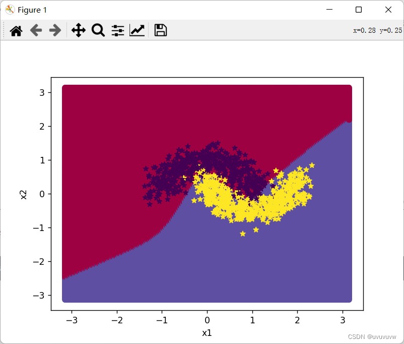
下面对结果进行可视化:
import math
import matplotlib.pyplot as plt
# 均匀生成40000个数据点
x1, x2 = torch.meshgrid(torch.linspace(-math.pi, math.pi, 200), torch.linspace(-math.pi, math.pi, 200))
x = torch.stack([torch.flatten(x1), torch.flatten(x2)], 1)

# 预测对应类别
y = runner.predict(x)
y = torch.squeeze((y>=0.5).to(torch.float32),-1)

# 绘制类别区域
plt.ylabel('x2')
plt.xlabel('x1')
plt.scatter(x[:,0].tolist(), x[:,1].tolist(), c=y.tolist(), cmap=plt.cm.Spectral)

plt.scatter(X_train[:, 0].tolist(), X_train[:, 1].tolist(), marker='*', c=torch.squeeze(y_train,-1).tolist())
plt.scatter(X_dev[:, 0].tolist(), X_dev[:, 1].tolist(), marker='*', c=torch.squeeze(y_dev,-1).tolist())
plt.scatter(X_test[:, 0].tolist(), X_test[:, 1].tolist(), marker='*', c=torch.squeeze(y_test,-1).tolist())
plt.show()
结果如图:
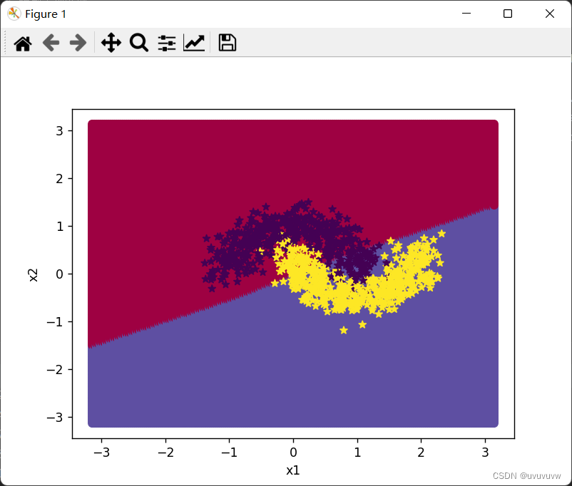
由图看出,直线不能很好的分类,提升学习率,将学习率提升至2
learning_rate = 2结果:
【思考题】对比3.1基于Logistic回归的二分类任务和 4.2 基于前馈神经网络的二分类任务谈谈自己的看法
logistic回归和神经网络都是二者都是基于最小化损失函数的思想,利用梯度下降法求导来更新权重参数。
logistic回归所有参数的更新是基于相同的式子,也就是所有参数的更新是基于相同的规则。 相比之下,神经网络每两个神经元之间参数的更新都基于不同式子,也就是每个参数的更新都是用不同的规则。
总结
本次实验对之前学过的反向传播算法加深了理解,更深刻了解了学习率对模型训练中的影响。


 1424
1424


 被折叠的 条评论
为什么被折叠?
被折叠的 条评论
为什么被折叠?
 到【灌水乐园】发言


