【点云处理之论文狂读前沿版5】APP-Net: Auxiliary-point-based Push and Pull Operations for Efficient Point Cloud Cls

Operations for Efficient Point Cloud Classification)

摘要

• 问题：在之前的工作中，基于点云的3D分类任务都设计从neighbor points中聚合特征，source point都会根据center point被选择成为neighbor points。这样就会不可避免地造成两个问题：
  (1)source point要参加多次运算，消耗大量的内存
  (2)依赖复杂的特征聚合器，降低网络的运行速度
• 解决方法：APP-Net，一个具有线性复杂度的特征聚合器
• 技术细节：
  (1)引入一个auxiliary container作为anchor来对source point和center point进行特征交换
  (2)每个source point都将其特征push到一个auxiliary container中，然后center point都会从auxiliary container中pull特征
  (3)使用一个在线法向量计算模块为网络提供二外的集合信息

1.引言

• 目前ModelNet40的分类精确度已经饱和了，现在需要研究的就是如何在保持较高精确度的同时还要降低计算复杂度和内存消耗。
• 在欧式距离下相近的点会被自动划分到相同的container中，container的维护开销很小
• APP的开销与输入点的数量成正比

2.相关工作

Multi-view Based Methods

Point Based Methods

3.方法

3.1Motivation and Discussion

P = { p 1 , p 2 , … , p N } \mathbf{P}=\left\{\mathbf{p}_{1}, \mathbf{p}_{2}, \ldots, \mathbf{p}_{N}\right\} P={p1​,p2​,…,pN​}表示 $N$ 个source points， Q = { q 1 , q 2 , … , q M } \mathbf{Q}=\left\{\mathbf{q}_{1}, \mathbf{q}_{2}, \ldots, \mathbf{q}_{M}\right\} Q={q1​,q2​,…,qM​}表示center points，局部点特征的聚合过程可以表示为：
g i = R ( { G ( r ( q i , p j , [ f i , f j ] ) , f j ) ∣ p j ∈ N ( q i ) } ) \mathbf{g}_{i}=R\left(\left\{G\left(r\left(\mathbf{q}_{i}, \mathbf{p}_{j},\left[\mathbf{f}_{i}, \mathbf{f}_{j}\right]\right), \mathbf{f}_{j}\right) \mid \mathbf{p}_{j} \in N\left(\mathbf{q}_{i}\right)\right\}\right) gi​=R({G(r(qi​,pj​,[fi​,fj​]),fj​)∣pj​∈N(qi​)})
其中${\mathbf{q}}_i$是center point，${\mathbf{g}}_i$是center point的输出特征，$N\left({\mathbf{q}}_i\right)$ 表示寻找${\mathbf{q}}_i$的neighbor points，${\mathbf{f}}_{\ast }\in {\mathbb{R}}^{C_{in}}$表示${\mathbf{p}}_{\ast }$ 或 ${\mathbf{q}}_{\ast }$的输入特征， $r\left({\mathbf{q}}_i,{\mathbf{p}}_j,\left[{\mathbf{f}}_i,{\mathbf{f}}_j\right]\right)$表示测量neighbour point和center point之间的关系，主要是位置关系和特征关系。$G$ 表示特征变换，$R$表示reduction操作（大部分情况下是max pooling）。

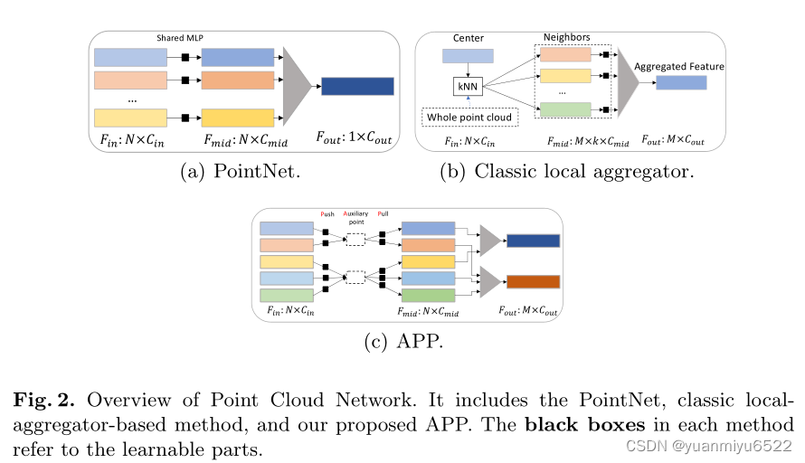
我们注意到，之前的方法都是从center point的角度聚合特征，每个center point也不考虑其他center points与自己的neighbor point相互处理了多少次。所以才提出了APP（auxiliary-based push and pull）网络，每个source point只进行一次特征处理，center point仅参与一次特征聚合。

尽管APP减少了网络的开销，但是auxiliary points也不可避免地引入了一些artifacts，因此我们引入了配对操作：
$$\gamma (x,y)=\alpha (x,\ast )?\beta (\ast ,y)$$
其中 $?$表示一种操作。

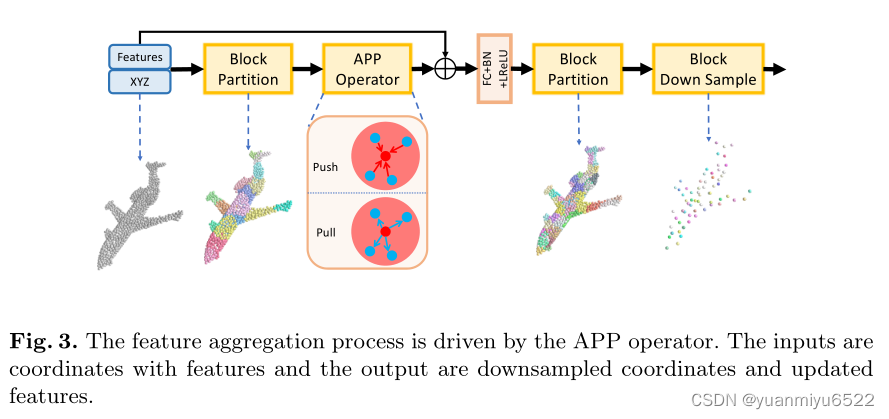
3.2 Auxiliary-based Push and Pull Operations

Block Partition

$\mathbf{A}=\left\{{\mathbf{a}}_0,{\mathbf{a}}_1,\dots ,{\mathbf{a}}_{\frac{N}{r_a}}\right\}$表示点云$\mathbf{P}$ 在采样率$r_a$下地子集。遵循RandLA-Net，本文采用随机采样，目的是为了节省时间。对于每个source point，我们采用 1-NN地方式从auxiliary point set $\mathbf{A}$中寻找auxiliary point，$A\left({\mathbf{p}}_i\right)$表示auxiliary point，在欧式空间上离得比较近地两个点很有可能被分配到相的auxiliary point。最终，全部的点云会被划分成几个不重叠的blocks $\left\{B\left({\mathbf{a}}_0\right),B\left({\mathbf{a}}_1\right),\dots ,B\left({\mathbf{a}}_{\frac{N}{r_a}}\right)\right\}$，其中$B\left({\mathbf{a}}_i\right)$表示source point set，1-NN auxiliary point为${\mathbf{a}}_i$。

Feature Aggregation

考虑一个基本公式：
$$e^{x-y}=e^{x-\ast +\ast -y}=e^{x-\ast }\cdot e^{\ast -y}$$
因此使用指数函数可以构造上面哪个方程组 { α , β , γ } \{\alpha, \beta, \gamma\} {α,β,γ}，整体的特征聚合步骤包含两步：Push-step 和 Pull-step

Push-step

在这一步中，source point的信息通过下式传递到auxiliary point中：
$${\mathbf{g}}_{{\mathbf{p}}_i\to A\left({\mathbf{p}}_i\right)}={\mathbf{f}}_i\cdot e^{W\times \left[\varphi \left({\mathbf{p}}_i\right)-\varphi \left(A\left({\mathbf{p}}_i\right)\right)\right]}$$
其中$\varphi (\ast )$ 是[FCLayer + BatchNorm + Leaky ReLU]形式的全局共享位置编码方程，他将3通道的向量提升到了$C_{in}$个通道。$W\in {\mathbb{R}}^{C_{in}\times C_{in}}$是一个可学习的权重矩阵。$\cdot$表示元素间的乘法，$\times$表示矩阵乘法。该过程根据空间关系将source point push到auxiliary point中去。

值得注意的是，属于相同auxiliary point的source point都会将他们的特征push到该auxiliary point中，因此该auxiliary point的最终特征应为：

$$\begin{gathered} {\mathbf{g}}_{A\left({\mathbf{p}}_i\right)}=\frac{1}{\left|B\left(A\left({\mathbf{p}}_i\right)\right)\right|}\sum _{{\mathbf{p}}_j\in \\ B\left(A\left({\mathbf{p}}_i\right)\right)}{\mathbf{f}}_j\cdot e^{W\times \left[\varphi \left({\mathbf{p}}_j\right)-\varphi \left(A\left({\mathbf{p}}_i\right)\right)\right]}. \end{gathered}$$

Pull-step

每一个auxiliary point都通过Push-step操作聚合block信息。在这个步骤中，利用利用逆向操作来为source point 从对应的auxiliary point中pull出特征：
$$\begin{gathered} {\mathbf{g}}_i={\mathbf{g}}_{A\left({\mathbf{p}}_i\right)\to {\mathbf{p}}_i}, \\ ={\mathbf{g}}_{A\left({\mathbf{p}}_i\right)}\cdot e^{W\times \left[\varphi \left(A\left({\mathbf{p}}_i\right)\right)-\varphi \left({\mathbf{p}}_i\right)\right]}, \\ =\left\{\frac{1}{\left|B\left(A\left({\mathbf{p}}_i\right)\right)\right|}\sum _{{\mathbf{p}}_j\in \\ B\left(A\left({\mathbf{p}}_i\right)\right)}{\mathbf{f}}_j\cdot e^{W\times \left[\varphi \left({\mathbf{p}}_j\right)-\varphi \left(A\left({\mathbf{p}}_i\right)\right)\right]}\right\}\cdot e^{W\times \left[\varphi \left(A\left({\mathbf{p}}_i\right)\right)-\varphi \left({\mathbf{p}}_i\right)\right]}, \\ =\frac{1}{\left|B\left(A\left({\mathbf{p}}_i\right)\right)\right|}\sum _{{\mathbf{p}}_j\in \\ B\left(A\left({\mathbf{p}}_i\right)\right)}{\mathbf{f}}_j\cdot e^{W\times \left[\varphi \left({\mathbf{p}}_j\right)-\varphi \left({\mathbf{p}}_i\right)\right]}. \end{gathered}$$

从本质上来讲，上式是将第一个式子中的reduction操作替换为Mean pooling得到的。Push-step 和 Pull-step操作共享相同的权重矩阵$W$h和编码函数$\varphi (\ast )$，auxiliary point的影响就会被减少，因此没有必要执行$\varphi \left(A\left({\mathbf{p}}_i\right)\right)$ ，The auxiliary point仅仅影响着${\mathbf{g}}_i$的感知域。此外，由于$e^{W\times \left[\varphi \left(A\left({\mathbf{p}}_i\right)\right)-\varphi \left({\mathbf{p}}_i\right)\right]}=\frac{1}{e^{W\times \left[\varphi \left({\mathbf{p}}_i\right)-\varphi \left(A\left({\mathbf{p}}_i\right)\right)\right]}}$，因此在等式4中计算到的空间信息可以直接用到等式6中。

那么最后的特征可以被更新为：

$${\mathbf{g}}_i^{\text{final }}=\delta \left(\left[{\mathbf{g}}_i,{\mathbf{f}}_i\right]\right).$$
其中$\delta (\ast )$是一个非线性函数，通过 { F C + \{\mathrm{FC}+ {FC+ BatchNorm $+$ LeakyReLU $\}$构造而成，${\mathbf{g}}_i^{\text{final }}\in {\mathbb{R}}^{C_{\text{out }}}$。

Block-based Down Sample

在处理完Push-step and Pull-step操作后，点云仍有 $N$ 个点，我们设计了Block-based Down Sample策略进一步减少中间的开销。

• 以${\mathbf{r}}_d$的为概率对点云进行下采样，然后基于1-NN算法将全部点分成不重叠的blocks $\left\{{\mathbf{D}}_0,{\mathbf{D}}_1,\dots ,{\mathbf{D}}_{\frac{N}{{\mathbf{r}}_d}}\right\}$
• 对于所有属于相同block ${\mathbf{D}}_i$的点，通过 Max pooling函数将他们的特征进行聚合：
  g d i = M A X { f j ∣ p j ∈ D i } \mathbf{g}_{\mathbf{d}_{i}}=M A X\left\{\mathbf{f}_{j} \mid \mathbf{p}_{j} \in \mathbf{D}_{i}\right\} gdi​​=MAX{fj​∣pj​∈Di​}

3.3Local Geometry by Online Normal and Curvature Estimation

本文利用最简单的 PCA 方法计算法向量，对于centroid point $\mathbf{p}$，通过下式组成其局部协方差矩阵：
C o v = 1 ∣ N ( p ) ∣ ∑ p i ∈ N ( p ) ( p i − p ) ⋅ ( p i − p ) , C o v ⋅ v j → = λ j ⋅ v j → , j ∈ { 0 , 1 , 2 } Cov=\frac{1}{|N(\mathbf{p})|} \sum_{\mathbf{p}_{i} \in N(\mathbf{p})}\left(\mathbf{p}_{i}-\mathbf{p}\right) \cdot\left(\mathbf{p}_{i}-\mathbf{p}\right), Cov \cdot \overrightarrow{v_{j}}=\lambda_{j} \cdot \overrightarrow{v_{j}}, j \in\{0,1,2\} Cov=∣N(p)∣1​pi​∈N(p)∑​(pi​−p)⋅(pi​−p),Cov⋅vj​ ​=λj​⋅vj​ ​,j∈{0,1,2}

${\vec{v}}_{\ast }$和${\lambda }_{\ast }$分别表示协方差矩阵的特征向量和特征值。最小特征值所对应的特征向量${\vec{v}}_{\ast }$是计算得到的法向量。假设${\lambda }_0$是最小特征向量，那么局部表面的曲率$\sigma$可以表示为
$$\sigma =\frac{{\lambda }_0}{{\lambda }_0+{\lambda }_1+{\lambda }_2}$$

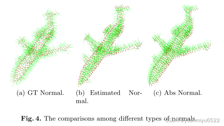
方向一致性检验将会使哪些没有指向预先设定视点
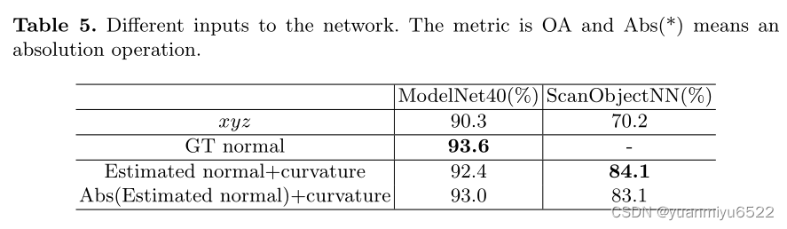
的法向量反转，从而减少歧义性。为了进一步减少噪声的影响，我们利用了一个==暴力 abs==操作保证所计算的法向量都是非负的。最终的向量在物理意义上不再是法向量。

3.4 The Full Structure of APP-Net

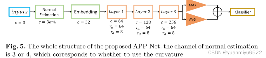
输入是点云信息，包括坐标 $xyz$，法向量，曲率（可选）。Embedding layer将输入的法向量（或是曲率）的维度提升至32。接下来的三层包含了APP operator 和 blocks down sample，用于聚合每个点的邻域特征。在最后的APP layer后，pooling layer输出全局特征，根据全局特征，包含了 MLPs的分类器将会预测每个类别的概率。

4.实验

4.1 Settings

• one Tesla V100 GPU
• PyTorch
• Adam
• cosine learning rate scheduler
• Initial learning rate = 2e-3，threshold = 2e-4
• 300 epochs with training batch size=32 and test batch size=16

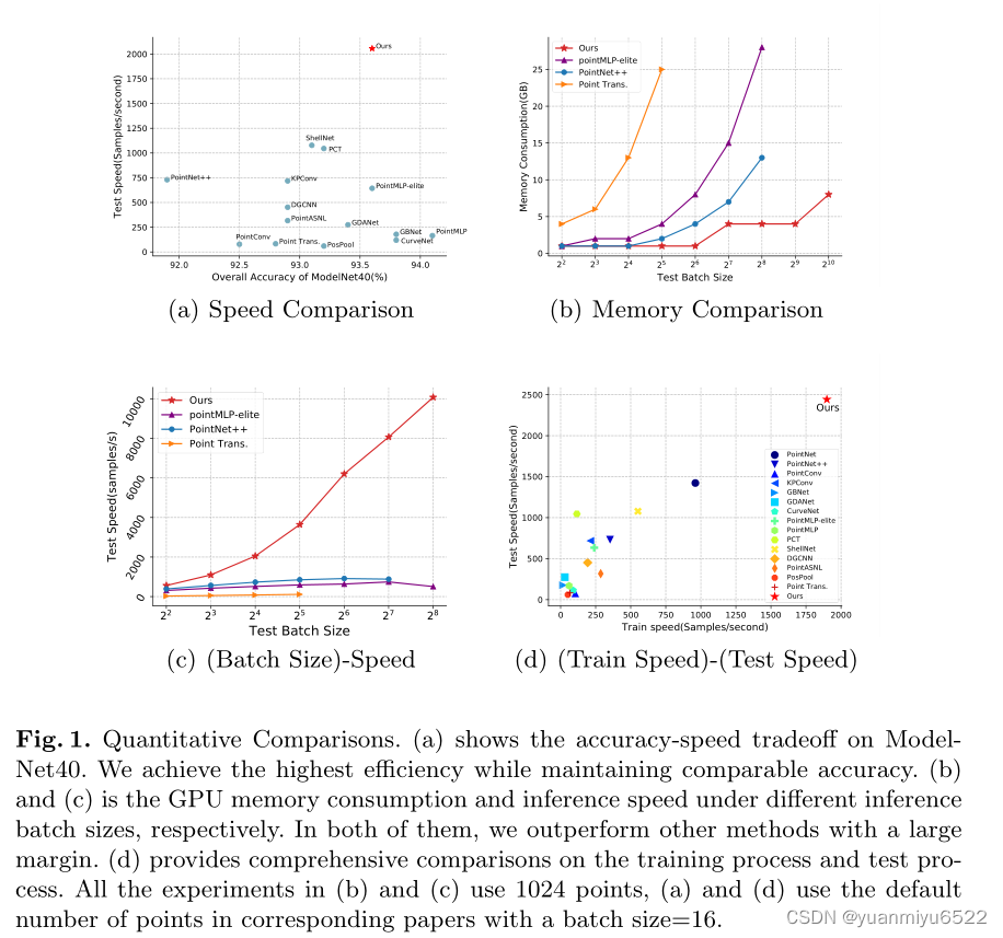
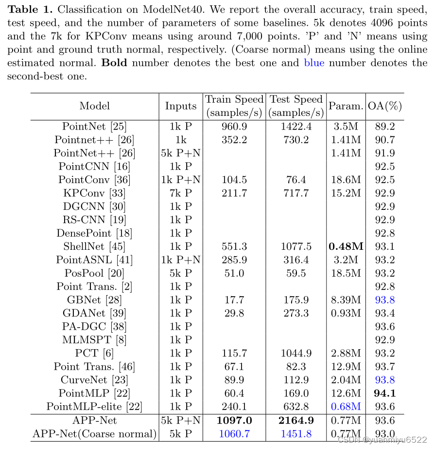
4.2 Shape Classification on ModelNet40

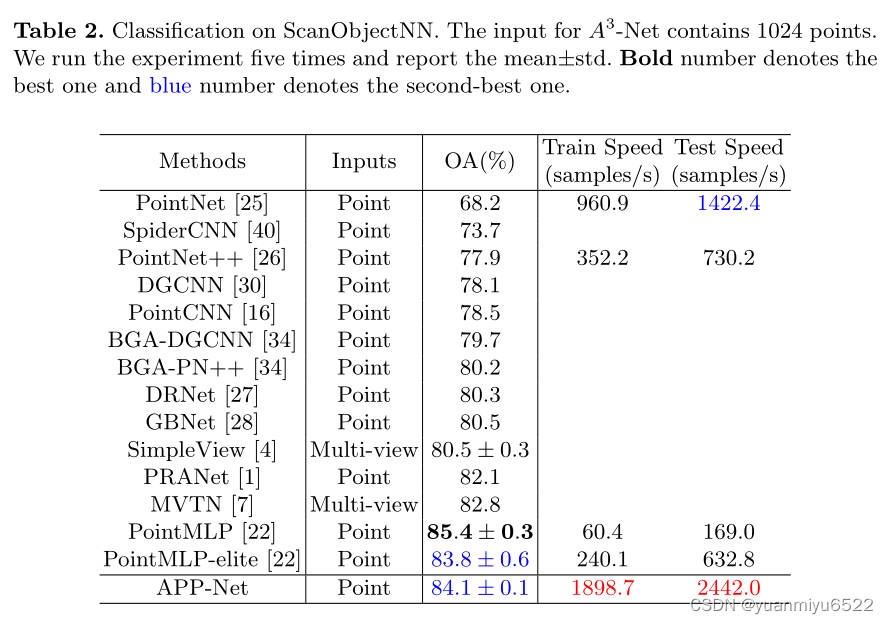
4.3 Shape Classification on ScanObjectNN (PB T50 RS)

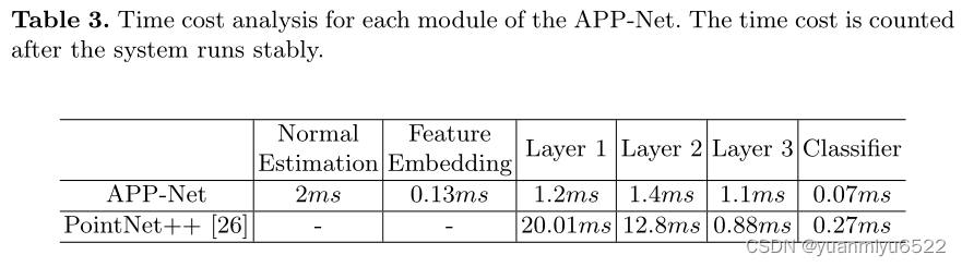
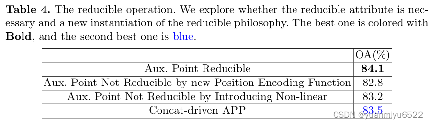
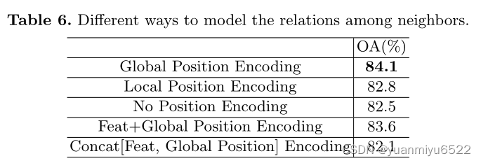
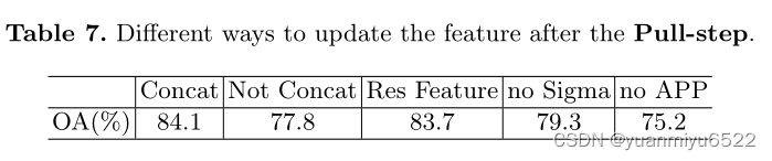
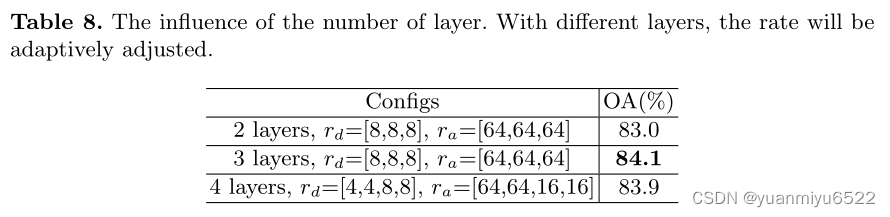
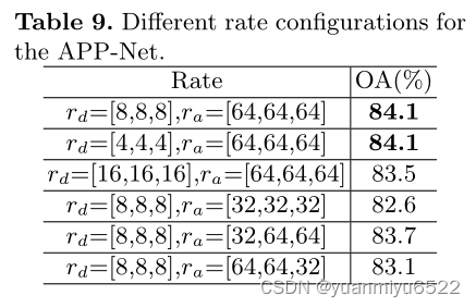
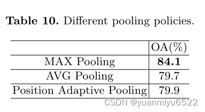
4.4 Ablation Studies

5.结论

本文的特色就是内存消耗少，处理速度快！