ALSA docs - Programming and Using Linux Sound - in depth

http://wiki.linuxaudio.org/wiki/tutorials/start

General

• The KXStudio manual serves as a good introduction to Linux Audio in general.
• Introduction to Linux & Audio by Lieven Moors
• A list of on-line articles by Dave Phillips
• An ebook on Linux Audio Programming by Jan Newmarch

 

 

-----------Programming and Using Linux Sound -  in depth----------------

Basic concepts of sound

This chapter looks at some basic concepts of audio, both analogue and digital.     

skip table of contents

Show table of contents

• Resources
• Sampled audio
• Sample rate
• Sample format
• Frames
• Pulse-code modulation
• Over and Under Run
• Latency
• Jitter
• Mixing
• Conclusion

Resources

1.   The Scientist and Engineer's Guide to   Digital Signal Processing by Steven W Smith        Digital Image Basics by      
2.   Music and Computers - A Theoretical and Historical Approach by Phil Burk, SoftSynth.com Larry Polansky, Department of Music, Dartmouth College Douglas Repetto, Computer Music Center, Columbia University Mary Roberts Dan Rockmore, Department of Mathematics, Dartmouth College     

Sampled audio

      Audio is an analogue phenomenon. Sounds are produced in all sorts      of ways, through voice, instruments and natural events such as trees      falling in forests (whether or not there is anyone to hear).       Sounds received at      a point can be plotted as amplitude against time and can assume      almost any functional state, including discontuous.   

      The analysis of sound is frequently done by looking at its      spectrum. Mathematically this is achieved by taking the Fourier      transform, but the ear performs almost a similar transform      just by the structure of the ear. "Pure" sounds heard by the ear      correspond to simple sine waves, and harmonics correspond to      sine waves which have a frequency a multiple of the base sine wave.   

      Analogue signals within a system such as an analogue audio amplifier      are designed to work with these spectral signals. They try to produce      an equal amplification across the audible spectrum.   

      Computers, and an increasingly large number of electronic devices,      work on digital signals, comprised of bits of ones and zeroes. Bits      are combined into bytes with 256 possible values, or 16 bit words      with 65536 possible values, or even larger combinations such as      32 or 64 bit words.   

Sample rate

      Digitising an analogue signal means taking samples from that signal      at regular intervals, and representing those samples on a discrete      scale. The frequency of taking samples is the sample rate.      For example, audio on a CD is sampled at 44,100hz, that is,       44,100 times each second. On a DVD, samples may be taken      upto 192,000 times per second, with a sampling rate of      192kHz. Conversely, the standard telephone sampling rate      is 8hhz.   

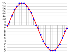
      This figure from      Wikipedia: Pulse-code modulation            illustrates sampling:     

      The sampling rate affects two major factors. Firstly, the      higher the sampling rate, the larger the size of the data.      All other things being equal, doubling the sample rate      will double the data requirements.      On the other hand the      Nyquist-Shannon theorem            places limits on the accuracy of sampling continous data:      an analogue signal can only be reconstructed from a digital      signal (i.e. be distortion-free) if the highest frequency      in the signal is less than one-half the sampling rate.   

      This is often where the arguments about the "quality" of      vinyl versus CDs end up, as in      Vinyl vs. CD myths refuse to die      .      With a sampling rate of 44.1kHz, frequencies in the original      signal above 22.05kHz may not be reproduced accurately when      converted back to analogue for a loudspeaker or headphones.      Since the typical hearing range for humans is only upto 20,000hz      (and mine is now down to about 10,000hz) then this should not be      a significant problem. But some audiophiles claim to have amazingly      sensitive ears...   

Sample format

      The sample format is the other major feature of digitizing      audio: the number of bits used to discretize the sample.      For example, telephone signals use 8kHz sampling rate and      8-bit resolution (see      How Telephones Work      ) so that a telephone signal can only convey      2^8 i.e. 256 levels.   

      Most CDs and computer systems use 16-bit formats.      (see      Audacity - Digital Sampling       )      giving a very fine gradation of the signal and allowing      a range of 96dB.   

Frames

      A frame holds all of the samples from one time instant.      For a stereo device, each frame holds two samples, while      for a five-speaker device, each frame would hold five samples.   

Pulse-code modulation

      Pulse-code modulation (PCM) is the standard form of representing a digitized      analogue signal.      From Wikipedia

  Pulse-code modulation (PCM) is a method used to digitally represent sampled analog signals.   It is the standard form for digital audio in computers and various   Blu-ray, DVD and Compact Disc formats, as well as other uses such   as digital telephone systems. A PCM stream is a digital representation   of an analog signal, in which the magnitude of the analog signal is   sampled regularly at uniform intervals, with each sample being   quantized to the nearest value within a range of digital steps.

  PCM streams have two basic properties that determine their fidelity   to the original analog signal: the sampling rate, which is the number   of times per second that samples are taken; and the bit depth, which   determines the number of possible digital values that each sample can take.

      However, even though this is the "standard", there are       variations      .      The principal one concerns the representation as bytes in a word-based system:      little-endian or big-endian      .      The next variation is       signed versus unsigned      .   

      There are a number of other variations which are less important,      such as whether the digitisation is linear or logarithmic.      See the     Multi-media Wikipedia      for discussion of these.   

Over and Under Run

      From Introduction to Sound Programming with ALSA     

      When a sound device is active, data is transferred continuously between       the hardware and application buffers. In the case of data capture (recording),       if the application does not read the data in the buffer rapidly enough,       the circular buffer is overwritten with new data. The resulting data       loss is known as overrun. During playback, if the application does not       pass data into the buffer quickly enough, it becomes starved for data,       resulting in an error called underrun.   

Latency

      Latency is the amount of time that elapses from when a signal      enters a system to when it (or its equivalent such as an amplified version)      leaves the system.   

      From Ian Waugh's Fixing Audio Latency Part 1:     

  Latency is a delay. It's most evident and problematic in computer-based music audio   systems where it manifests as the delay between triggering a signal and hearing it.   For example, pressing a key on your MIDI keyboard and hearing the sound play   through your sound card.

  It's like a delayed reaction and if the delay is very large it becomes impossible   to play anything in time because the sound you hear is always a little bit behind   what you're playing which is very distracting.

  This delay does not have to be very large before it causes problems.   Many people can work with a latency of about 40ms even though the delay is noticeable,   although if you are playing pyrotechnic music lines it may be too long.

  The ideal latency is 0 but many people would be hard pushed to notice delays of   less than 8-10ms and many people can work quite happily with a 20ms latency.

      A Google search for "measuring audio latency" will turn up many sites.      I use a crude - but simple - test. I installed Audacity on a separate PC,      and used it to record simultaneously a sound I made and that sound when       picked up and played back by the test PC. I banged a spoon against a bottle      to get a sharp percursive sound. When magnified, the recorded sound showed       two peaks and selecting the region between the peaks showed me the latency      in the selection start/end. In the figure below, these are      17.383 and 17.413 seconds, with a latency of 30 msecs.     

Jitter

      Sampling an analogue signal will be done at regular intervals.      Ideally, playback should use exactly those same intervals.      But, particularly in networked systems, the periods may not      be regular. Any irregularity is known as      jitter      .      I don't have a simple way of testing for jitter - I'm still stuck      on latency as my major problem!   

Mixing

      Mixing means taking inputs from one or more sources, possibly doing      some processing on these input signals and sending them to one or      more outputs. The origin, of course, is in physical mixers which      would act on analogue signals. In the digital world the same functions      would be performed on digital signals.   

      A simple document describing analogues mixers is      The Soundcraft Guide to Mixing      . This covers the functions of     

•   Routing inputs to outputs
•   Setting gain and output levels for different input and output signals
•   Applying special effects such as reverb, delay and pitch shifting
•   Mixing input signals to a common output
•   Splitting an input signal into multiple outputs

Conclusion

This short chapter has introduced some of the basic concepts that will occupy much of the rest of this book.   The Scientist and Engineer's Guide to   Digital Signal Processing by Steven W Smith has  wealth of further detail,     

 

 

 

 

 

Writing an ALSA Driver
		Next

---

Writing an ALSA Driver

Takashi Iwai

          <tiwai@suse.de>
       

    Copyright (c) 2002-2005  Takashi Iwai <tiwai@suse.de>

    This document is free; you can redistribute it and/or modify it    under the terms of the GNU General Public License as published by    the Free Software Foundation; either version 2 of the License, or    (at your option) any later version.    

    This document is distributed in the hope that it will be useful,    but WITHOUT ANY WARRANTY; without even the    implied warranty of MERCHANTABILITY or FITNESS FOR A    PARTICULAR PURPOSE. See the GNU General Public License    for more details.   

    You should have received a copy of the GNU General Public    License along with this program; if not, write to the Free    Software Foundation, Inc., 59 Temple Place, Suite 330, Boston,    MA 02111-1307 USA   

Abstract

        This document describes how to write an ALSA (Advanced Linux        Sound Architecture) driver.     

---

List of Examples

1.1. ALSA File Tree Structure 2.1. Basic Flow for PCI Drivers - Example 4.1. PCI Resource Management Example 5.1. PCM Example Code 5.2. PCM Instance with a Destructor 5.3. Interrupt Handler Case #1 5.4. Interrupt Handler Case #2 5.5. Example of Hardware Constraints 5.6. Example of Hardware Constraints for Channels 5.7. Example of Hardware Constraints for Channels 6.1. Definition of a Control 6.2. Example of info callback 6.3. Example of get callback 6.4. Example of put callback 7.1. Example of AC97 Interface 15.1. Sample Makefile for a driver xyz