NN Representational power && Setting number of layers and their sizes

One way to look at Neural Networks with fully-connected layers is that they define a family of functions that are parameterized by the weights of the network. A natural question that arises is: What is the representational power of this family of functions? In particular, are there functions that cannot be modeled with a Neural Network?

It turns out that Neural Networks with at least one hidden layer are universal approximators. That is, it can be shown (e.g. see Approximation by Superpositions of Sigmoidal Function from 1989 (pdf), or this intuitive explanation from Michael Nielsen) that given any continuous function  f(x) f(x) and some  ϵ>0 ϵ>0, there exists a Neural Network  g(x) g(x) with one hidden layer (with a reasonable choice of non-linearity, e.g. sigmoid) such that  ∀x,∣f(x)−g(x)∣<ϵ ∀x,∣f(x)−g(x)∣<ϵ. In other words, the neural network can approximate any continuous function.

If one hidden layer suffices to approximate any function, why use more layers and go deeper? The answer is that the fact that a two-layer Neural Network is a universal approximator is, while mathematically cute, a relatively weak and useless statement in practice. In one dimension, the “sum of indicator bumps” function  g(x)=∑ici1(ai<x<bi) g(x)=∑ici1(ai<x<bi) where  a,b,c a,b,c are parameter vectors is also a universal approximator, but noone would suggest that we use this functional form in Machine Learning. Neural Networks work well in practice because they compactly express nice, smooth functions that fit well with the statistical properties of data we encounter in practice, and are also easy to learn using our optimization algorithms (e.g. gradient descent). Similarly, the fact that deeper networks (with multiple hidden layers) can work better than a single-hidden-layer networks is an empirical observation, despite the fact that their representational power is equal.

As an aside, in practice it is often the case that 3-layer neural networks will outperform 2-layer nets, but going even deeper (4,5,6-layer) rarely helps much more. This is in stark contrast to Convolutional Networks, where depth has been found to be an extremely important component for a good recognition system (e.g. on order of 10 learnable layers). One argument for this observation is that images contain hierarchical structure (e.g. faces are made up of eyes, which are made up of edges, etc.), so several layers of processing make intuitive sense for this data domain.

The full story is, of course, much more involved and a topic of much recent research. If you are interested in these topics we recommend for further reading:

• Deep Learning book in press by Bengio, Goodfellow, Courville, in particular Chapter 6.4.
• Do Deep Nets Really Need to be Deep?
• FitNets: Hints for Thin Deep Nets

Setting number of layers and their sizes

How do we decide on what architecture to use when faced with a practical problem? Should we use no hidden layers? One hidden layer? Two hidden layers? How large should each layer be? First, note that as we increase the size and number of layers in a Neural Network, the capacity of the network increases. That is, the space of representable functions grows since the neurons can collaborate to express many different functions. For example, suppose we had a binary classification problem in two dimensions. We could train three separate neural networks, each with one hidden layer of some size and obtain the following classifiers:

Larger Neural Networks can represent more complicated functions. The data are shown as circles colored by their class, and the decision regions by a trained neural network are shown underneath. You can play with these examples in this  ConvNetsJS demo.

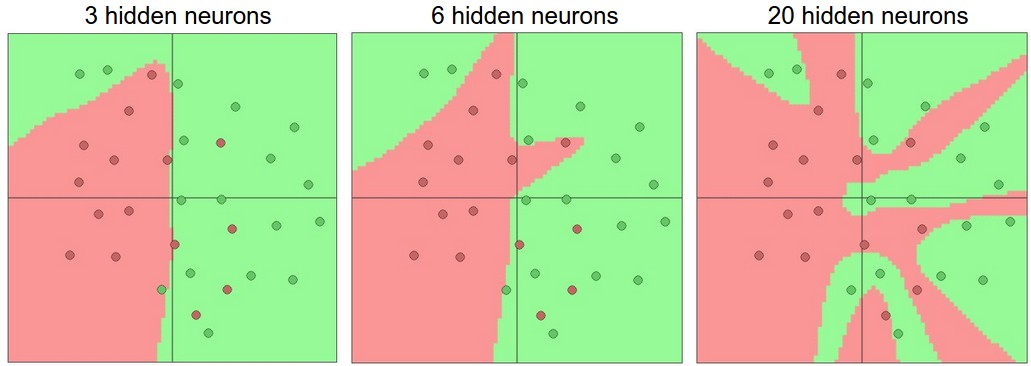
In the diagram above, we can see that Neural Networks with more neurons can express more complicated functions. However, this is both a blessing (since we can learn to classify more complicated data) and a curse (since it is easier to overfit the training data). Overfitting occurs when a model with high capacity fits the noise in the data instead of the (assumed) underlying relationship. For example, the model with 20 hidden neurons fits all the training data but at the cost of segmenting the space into many disjoint red and green decision regions. The model with 3 hidden neurons only has the representational power to classify the data in broad strokes. It models the data as two blobs and interprets the few red points inside the green cluster as outliers (noise). In practice, this could lead to better generalization on the test set.

Based on our discussion above, it seems that smaller neural networks can be preferred if the data is not complex enough to prevent overfitting. However, this is incorrect - there are many other preferred ways to prevent overfitting in Neural Networks that we will discuss later (such as L2 regularization, dropout, input noise). In practice, it is always better to use these methods to control overfitting instead of the number of neurons.

The subtle reason behind this is that smaller networks are harder to train with local methods such as Gradient Descent: It’s clear that their loss functions have relatively few local minima, but it turns out that many of these minima are easier to converge to, and that they are bad (i.e. with high loss). Conversely, bigger neural networks contain significantly more local minima, but these minima turn out to be much better in terms of their actual loss. Since Neural Networks are non-convex, it is hard to study these properties mathematically, but some attempts to understand these objective functions have been made, e.g. in a recent paper The Loss Surfaces of Multilayer Networks. In practice, what you find is that if you train a small network the final loss can display a good amount of variance - in some cases you get lucky and converge to a good place but in some cases you get trapped in one of the bad minima. On the other hand, if you train a large network you’ll start to find many different solutions, but the variance in the final achieved loss will be much smaller. In other words, all solutions are about equally as good, and rely less on the luck of random initialization.

To reiterate, the regularization strength is the preferred way to control the overfitting of a neural network. We can look at the results achieved by three different settings:

The effects of regularization strength: Each neural network above has 20 hidden neurons, but changing the regularization strength makes its final decision regions smoother with a higher regularization. You can play with these examples in this  ConvNetsJS demo.

The takeaway is that you should not be using smaller networks because you are afraid of overfitting. Instead, you should use as big of a neural network as your computational budget allows, and use other regularization techniques to control overfitting.