强化学习的学习之路（三十一）_2021-01-31： REINFORCE

作为一个新手，写这个强化学习-基础知识专栏是想和大家分享一下自己学习强化学习的学习历程，希望对大家能有所帮助。这个系列后面会不断更新，希望自己在2021年能保证平均每日一更的更新速度，主要是介绍强化学习的基础知识，后面也会更新强化学习的论文阅读专栏。本来是想每一篇多更新一点内容的，后面发现大家上CSDN主要是来提问的，就把很多拆分开来了（而且这样每天任务量也小一点哈哈哈哈偷懒大法）。但是我还是希望知识点能成系统，所以我在目录里面都好按章节系统地写的，而且在github上写成了书籍的形式，如果大家觉得有帮助，希望从头看的话欢迎关注我的github啊，谢谢大家！另外我还会分享深度学习-基础知识专栏以及深度学习-论文阅读专栏，很早以前就和小伙伴们花了很多精力写的，如果有对深度学习感兴趣的小伙伴也欢迎大家关注啊。大家一起互相学习啊！可能会有很多错漏，希望大家批评指正！不要高估一年的努力，也不要低估十年的积累，与君共勉！

REINFOECE

先回顾一下强化学习的目标，最大化累计奖励：

$${\theta }^{\star }=\arg \underset{\theta }{\max }{E}_{\tau \sim p_{\theta }(\tau )}\left[\sum _{t}r\left({\mathbf{s}}_t,{\mathbf{a}}_t\right)\right]$$

在有限长度轨迹的情况下：

$${\theta }^{\star }=\arg \underset{\theta }{\max }{E}_{(\mathbf{s},\mathbf{a})\sim p_{\theta }(\mathbf{s},\mathbf{a})}[r(\mathbf{s},\mathbf{a})]$$

在无限长度轨迹的情况下：

$${\theta }^{\star }=\arg \underset{\theta }{\max }\sum _{t=1}^T{E}_{\left({\mathbf{s}}_t,{\mathbf{a}}_t\right)\sim p_{\theta }\left({\mathbf{s}}_t,{\mathbf{a}}_t\right)}\left[r\left({\mathbf{s}}_t,{\mathbf{a}}_t\right)\right]$$

我们令目标函数：

$$J(\theta )=E_{\tau \sim p_{\theta }(\tau )}\left[\sum _{t}r\left({\mathbf{s}}_t,{\mathbf{a}}_t\right)\right]\approx \frac{1}{N}\sum _i\sum _{t}r\left({\mathbf{s}}_{i,t},{\mathbf{a}}_{i,t}\right)$$，令第一项中括号中的为$$r(\tau )$$，

$$\begin{array}{c}J(\theta )=E_{\tau \sim p_{\theta }(\tau )}[\underbrace{r(\tau )]}\hookrightarrow =\int p_{\theta }(\tau )r(\tau )d\tau \\ {\sum }_{t=1}^{T}r\left({\mathbf{s}}_t,{\mathbf{a}}_t\right)\end{array}$$

对它直接进行梯度计算:
$${\nabla }_{\theta }J(\theta )=\int {\nabla }_{\theta }{p}_{\theta }(\tau )r(\tau )d\tau =\int p_{\theta }(\tau ){\nabla }_{\theta }\log p_{\theta }(\tau )r(\tau )d\tau =E_{\tau \sim p_{\theta }(\tau )}\left[{\nabla }_{\theta }\log p_{\theta }(\tau )r(\tau )\right]$$
在这里的第二个等号中，使用了一个恒等式:

$$p_{\theta }(\tau ){\nabla }_{\theta }\log p_{\theta }(\tau )=p_{\theta }(\tau )\frac{{\nabla }_{\theta }{p}_{\theta }(\tau )}{p_{\theta }(\tau )}={\nabla }_{\theta }{p}_{\theta }(\tau )$$

而 $$\underset{p_{\theta }(\tau )}{\underbrace{p_{\theta }\left({\mathbf{s}}_1,{\mathbf{a}}_1,\dots ,{\mathbf{s}}_T,{\mathbf{a}}_T\right)}}=p\left({\mathbf{s}}_1\right)\prod _{t=1}{\pi }_{\theta }\left({\mathbf{a}}_t\mid {\mathbf{s}}_t\right)p\left({\mathbf{s}}_{t+1}\mid {\mathbf{s}}_t,{\mathbf{a}}_t\right)$$

两边取log：

$$\log p_{\theta }(\tau )=\log p\left({\mathbf{s}}_1\right)+\sum _{t=1}^T\log {\pi }_{\theta }\left({\mathbf{a}}_t\mid {\mathbf{s}}_t\right)+\log p\left({\mathbf{s}}_{t+1}\mid {\mathbf{s}}_t,{\mathbf{a}}_t\right)$$

所以：

$${\nabla }_{\theta }\log p_{\theta }(\tau )r(\tau )$$= $${\nabla }_{\theta }\left[\log /p\left({\mathbf{s}}_1\right)+\sum _{t=1}^T\log {\pi }_{\theta }\left({\mathbf{a}}_t\mid {\mathbf{s}}_t\right)+\log p\left({\mathbf{s}}_{t+1}\widehat{{\mathbf{s}}_t},{\mathbf{a}}_t\right)\right]$$

第一项和第三项都和$\theta$没有关系，所以

$${\nabla }_{\theta }J(\theta )=E_{\tau \sim p_{\theta }(\tau )}\left[{\nabla }_{\theta }\log p_{\theta }(\tau )r(\tau )\right]$$ = $$E_{\tau \sim p_{\theta }(\tau )}\left[\left(\sum _{t=1}^T{\nabla }_{\theta }\log {\pi }_{\theta }\left({\mathbf{a}}_t\mid {\mathbf{s}}_t\right)\right)\left(\sum _{t=1}^{T}r\left({\mathbf{s}}_t,{\mathbf{a}}_t\right)\right)\right]$$

​ $$\approx \frac{1}{N}\sum _{i=1}^N\left(\sum _{t=1}^T{\nabla }_{\theta }\log {\pi }_{\theta }\left({\mathbf{a}}_{i,t}\mid {\mathbf{s}}_{i,t}\right)\right)\left(\sum _{t=1}^{T}r\left({\mathbf{s}}_{i,t},{\mathbf{a}}_{i,t}\right)\right)$$

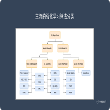
终于！这两项都可以通过采样然后通过样本算出来了！ 然后根据强化学习算法的经典的流程图：

我们就可以得到REINFORCE 算法，也就是根据当前策略进行采样，采样之后算出梯度，算出梯度之后对策略进行更新，然后继续采样，如此往复：

值得注意的是，在上述推导过程中，我们并没有用到Markov property，所以REINFORCE对partially observed MDPs而言也是可以使用的，因为它针对的是trajectory。

在离散动作空间下，可以跟分类任务一样，使用多个输出结点作为不同action的选择。

而在连续动作空间下，往往会使用Gaussian polices进行action选择：通过神经网络对state 进行处理，得到高斯分布的均值（方差可以得到也可以指定），再通过这个分布进行抽样。
$${\pi }_{\theta }\left({\mathbf{a}}_t\mid {\mathbf{s}}_t\right)=\mathcal{N}\left(f_{\text{neural network }}\left({\mathbf{s}}_t\right);\Sigma \right)$$
而由于高斯分布梯度易求，所以参数优化也比较方便
$$\begin{array}{l}\log {\pi }_{\theta }\left({\mathbf{a}}_t\mid {\mathbf{s}}_t\right)=-\frac{1}{2}{\Vert f\left({\mathbf{s}}_t\right)-{\mathbf{a}}_t\Vert }_{\Sigma }^2+\text{ const }\\ {\nabla }_{\theta }\log {\pi }_{\theta }\left({\mathbf{a}}_t\mid {\mathbf{s}}_t\right)=-\frac{1}{2}{\Sigma }^{-1}\left(f\left({\mathbf{s}}_t\right)-{\mathbf{a}}_t\right)\frac{df}{d\theta }\end{array}$$

上一篇：强化学习的学习之路（三十）_2021-01-30： Policy Optimazation 简介
下一篇：强化学习的学习之路（三十二）_2021-02-01：Differences between RL and Imitation learning（强化学习和模仿学习的差别）