Task05：数据建模及模型评估

一、模型搭建和评估

经过前面的探索性数据分析我们可以很清楚的了解到数据集的情况
导入库

import pandas as pd
import numpy as np
import seaborn as sns
import matplotlib.pyplot as plt
from IPython.display import Image
%matplotlib inline

plt.rcParams['font.sans-serif'] = ['SimHei']  # 用来正常显示中文标签
plt.rcParams['axes.unicode_minus'] = False  # 用来正常显示负号
plt.rcParams['figure.figsize'] = (10, 6)  # 设置输出图片大小

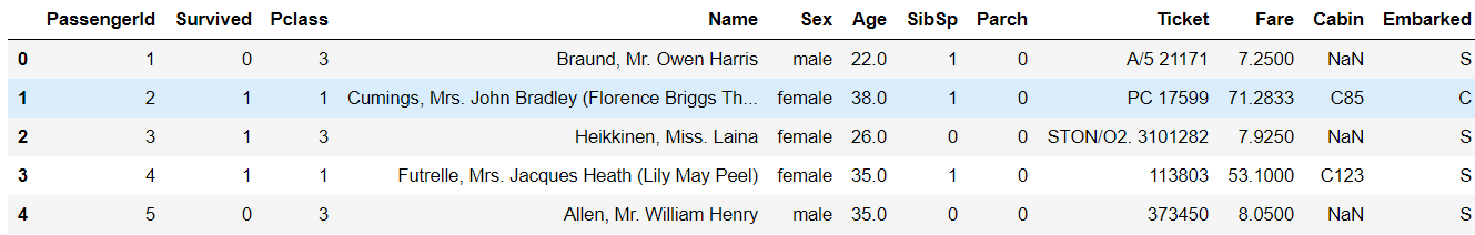
# 读取训练数集
train = pd.read_csv('train.csv')
print(train.shape)		# 输出结果为(891, 12)
print(train.head())		# 输出前5行

二、对缺失值进行填充

对分类变量缺失值：填充某个缺失值字符(NA)、用最多类别的进行填充
对连续变量缺失值：填充均值、中位数、众数

# 对分类变量进行填充
train['Cabin'] = train['Cabin'].fillna('NA')
train['Embarked'] = train['Embarked'].fillna('S')
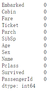
# 对连续变量进行填充
train['Age'] = train['Age'].fillna(train['Age'].mean())
# 检查缺失值比例
print(train.isnull().sum().sort_values(ascending=False))

三、编码分类变量

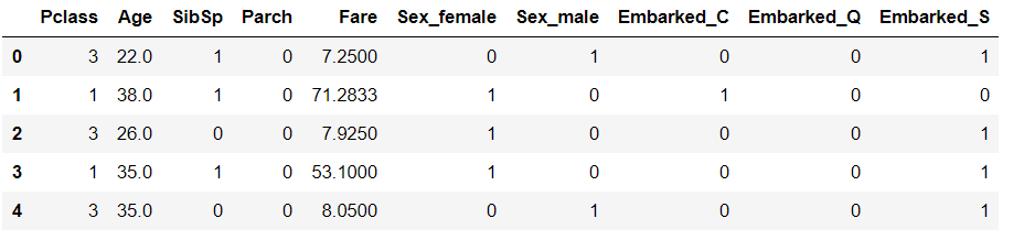
# 取出所有的输入特征
data = train[['Pclass','Sex','Age','SibSp','Parch','Fare', 'Embarked']]
# 进行虚拟变量转换
data = pd.get_dummies(data)
print(data.head())

四、模型搭建

from sklearn.model_selection import train_test_split
from sklearn.linear_model import LogisticRegression
from sklearn.ensemble import RandomForestClassifier
# 一般先取出X和y后再切割，有些情况会使用到未切割的，这时候X和y就可以用
X = data
y = train['Survived']
# 对数据集进行切割
X_train, X_test, y_train, y_test = train_test_split(X, y, stratify=y, random_state=0)
# 查看数据形状
print(X_train.shape, X_test.shape)  # ((668, 10), (223, 10))
# 默认参数逻辑回归模型
lr = LogisticRegression()
print(lr.fit(X_train, y_train))

LogisticRegression(C=1.0, class_weight=None, dual=False, fit_intercept=True,
intercept_scaling=1, max_iter=100, multi_class=‘ovr’, n_jobs=1,
penalty=‘l2’, random_state=None, solver=‘liblinear’, tol=0.0001,
verbose=0, warm_start=False)

# 查看训练集和测试集score值
print("Training set score: {:.2f}".format(lr.score(X_train, y_train)))   # Training set score: 0.80
print("Testing set score: {:.2f}".format(lr.score(X_test, y_test)))  #Testing set score: 0.78

# 调整参数后的逻辑回归模型
lr2 = LogisticRegression(C=100)
lr2.fit(X_train, y_train)

LogisticRegression(C=100, class_weight=None, dual=False, fit_intercept=True,
intercept_scaling=1, max_iter=100, multi_class=‘ovr’, n_jobs=1,
penalty=‘l2’, random_state=None, solver=‘liblinear’, tol=0.0001,
verbose=0, warm_start=False)

print("Training set score: {:.2f}".format(lr2.score(X_train, y_train)))
# Training set score: 0.80
print("Testing set score: {:.2f}".format(lr2.score(X_test, y_test)))
# Testing set score: 0.79
# 默认参数的随机森林分类模型
rfc = RandomForestClassifier()
rfc.fit(X_train, y_train)

RandomForestClassifier(bootstrap=True, class_weight=None, criterion=‘gini’,
max_depth=None, max_features=‘auto’, max_leaf_nodes=None,
min_impurity_decrease=0.0, min_impurity_split=None,
min_samples_leaf=1, min_samples_split=2,
min_weight_fraction_leaf=0.0, n_estimators=10, n_jobs=1,
oob_score=False, random_state=None, verbose=0,
warm_start=False)

print("Training set score: {:.2f}".format(rfc.score(X_train, y_train)))
# Training set score: 0.97
print("Testing set score: {:.2f}".format(rfc.score(X_test, y_test)))
# Testing set score: 0.82
# 调整参数后的随机森林分类模型
rfc2 = RandomForestClassifier(n_estimators=100, max_depth=5)
rfc2.fit(X_train, y_train)

RandomForestClassifier(bootstrap=True, class_weight=None, criterion=‘gini’,
max_depth=5, max_features=‘auto’, max_leaf_nodes=None,
min_impurity_decrease=0.0, min_impurity_split=None,
min_samples_leaf=1, min_samples_split=2,
min_weight_fraction_leaf=0.0, n_estimators=100, n_jobs=1,
oob_score=False, random_state=None, verbose=0,
warm_start=False)

print("Training set score: {:.2f}".format(rfc2.score(X_train, y_train)))
# Training set score: 0.86
print("Testing set score: {:.2f}".format(rfc2.score(X_test, y_test)))
# Testing set score: 0.83

五、输出预测结果

# 预测标签
pred = lr.predict(X_train)
# 此时我们可以看到0和1的数组
pred[:10]
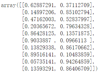
# 预测标签概率
pred_proba = lr.predict_proba(X_train)
print(pred_proba[:10])

六、模型评估

模型评估是为了知道模型的泛化能力。
交叉验证（cross-validation）是一种评估泛化性能的统计学方法，它比单次划分训练集和测试集的方法更加稳定、全面。
在交叉验证中，数据被多次划分，并且需要训练多个模型。
最常用的交叉验证是 k 折交叉验证（k-fold cross-validation），其中 k 是由用户指定的数字，通常取 5 或 10。
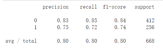
准确率（precision）度量的是被预测为正例的样本中有多少是真正的正例
召回率（recall）度量的是正类样本中有多少被预测为正类
f-分数是准确率与召回率的调和平均；

from sklearn.model_selection import cross_val_score
lr = LogisticRegression(C=100)
scores = cross_val_score(lr, X_train, y_train, cv=10)
# k折交叉验证分数
print(scores)

array([0.82352941, 0.79411765, 0.80597015, 0.80597015, 0.8358209 ,
0.88059701, 0.72727273, 0.86363636, 0.75757576, 0.71212121])

# 平均交叉验证分数
print("Average cross-validation score: {:.2f}".format(scores.mean()))
# Average cross-validation score: 0.80

混淆矩阵

from sklearn.metrics import confusion_matrix
# 训练模型
lr = LogisticRegression(C=100)
lr.fit(X_train, y_train)

LogisticRegression(C=100, class_weight=None, dual=False, fit_intercept=True,
intercept_scaling=1, max_iter=100, multi_class=‘ovr’, n_jobs=1,
penalty=‘l2’, random_state=None, solver=‘liblinear’, tol=0.0001,
verbose=0, warm_start=False)

# 模型预测结果
pred = lr.predict(X_train)
# 混淆矩阵
confusion_matrix(y_train, pred)

array([[350, 62],
[ 71, 185]], dtype=int64)

from sklearn.metrics import classification_report
# 精确率、召回率以及f1-score
print(classification_report(y_train, pred))

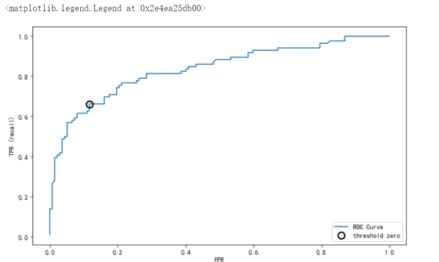
7、如何绘制ROC曲线

from sklearn.metrics import roc_curve
fpr, tpr, thresholds = roc_curve(y_test, lr.decision_function(X_test))
plt.plot(fpr, tpr, label="ROC Curve")
plt.xlabel("FPR")
plt.ylabel("TPR (recall)")
# 找到最接近于0的阈值
close_zero = np.argmin(np.abs(thresholds))
plt.plot(fpr[close_zero], tpr[close_zero], 'o', markersize=10, label="threshold zero", fillstyle="none", c='k', mew=2)
plt.legend(loc=4)